Section 4: Technical Calculations for the Capital and Leverage Tax Recommendations

This section provides the technical details behind our calculations used to support and define our capital and leverage tax recommendations.

Calculations Supporting Capital Requirement Recommendations

We make two calculations to support the capital recommendations that we describe in more detail in this section. First, we calculate the benefits of higher capital requirements. Second, we calculate the costs of higher capital requirements. We now provide a more technical discussion of our analysis than in Section 3.

Calculating the benefits of higher capital requirements

We estimate the benefits of the Minneapolis Plan using the IMF database of past banking crises and nonperforming loan (NPL) rates. To measure the number of crises avoided by particular capital ratio levels in this database, we must convert NPLs to losses and then to equivalent capital ratios. For a given capital ratio, the percentage of crises avoided can then be converted to an annualized bailout probability as well as a 100-year bailout probability.

As noted above, we follow DDLRT to calculate losses as a share of estimated risk-weighted assets. We utilize their measurements of peak NPLs for the crises in their database. NPL rates are converted to loss rates by multiplying by LGD. DDLRT adjust these loss rates further by using an estimate of prior loss provisioning and an uncertainty buffer. Loss provisioning is measured as a share of loans and is meant to capture how an average firm might prepare for expected losses. The uncertainty buffer is simply used to account for some of the uncertainty in this calculation. The rates are then converted to a capital ratio by multiplying by an estimate of the ratio of total assets to risk-weighted assets (RWA). This final step sets the ratio in terms of risk-based capital needs.

We operationalize the DDLRT NPL conversion using the following equation per the description above (except for LGD, whose derivation was already discussed). The formulas and numerical values below come from DDLRT.

Adjusted Losses/RWA	= (NPL × LGD – provisions + buffer) × (RWA conversion)
where
LGD	= Loss given default of 62.5%
provisions	= Prior provisioning equal to 1.5% of the loan base
buffer	= A 1% “safety buffer” to account for parameter uncertainty
RWA conversion	= A factor of 1.75

Inserting these values into the equation above, the final version of the DDLRT approach we use to convert NPLs into capital ratios is then:

Implied Capital Ratio

= Adjusted Losses/RWA = (NPL × 0.625 – 1.5 + 1.0) × (1.75)

We can now determine the number of crises avoided in the IMF database given a particular capital target. We further transform the number avoided to an annual bailout probability by multiplying the percentage of crises avoided by the unconditional probability of a crisis in the database. The unconditional probability of a crisis for OECD countries is approximately 3 percent.⁴⁰ Finally, we transform the annual bailout probabilities into 100-year bailout probabilities:

Annual Chance of a Bailout	= (1-% of crises avoided) × Probability of a crisis
Probability of Bailout over the next 100 years	= 1-(1 – Annual Chance of a Bailout)100

Calculating the costs of higher capital

We measure the cost of higher capital requirements in terms of lost GDP due to tighter lending conditions. This calculation requires a number of steps. We trace the impact of higher capital requirements to lower bank return on equity (ROE) and then to higher loan rates. Higher loan rates slow economic growth by restricting borrowing. As noted above, this approach closely follows the BIS.

In response to higher required capital levels, we assume that banks issue more equity and raise income by increasing their lending rates. To gauge the magnitudes of these changes, we proceed as follows:

• We first calculate the amount of equity that domestic covered banks will have to issue under a 23.5 percent CET1 capital standard by obtaining their equity levels as of fourth quarter 2015 from regulatory reports (the Y-9C) and subtracting that level from the mandated minimum level we are analyzing.
• Next, we determine the cost of issuing additional equity by assuming that covered banks pass through half of the higher costs of equity by increasing interest rates. At the same time, they suffer a decline in their ROE in order to make up the rest. The additional cost is borne by the covered banks in the form of lower net income.

This step requires us to gather information on both the ROE and the cost of debt as firms will be replacing existing liabilities with higher-cost equity as well as losing net income.

• ROE
  We obtain data on ROE from FactSet Data Systems. We calculate the median annual ROE for each covered bank in the 2010 to 2015 time period.  We then calculate the asset-weighted average to use as an approximation of covered bank ROE.
• Cost of Debt
  We obtain daily average credit spreads across all outstanding debt collected in the Moody’s KMV database for each year from 2010 to 2015. We also obtain daily average five-year CMT rates from the St. Louis Fed (FRED) database in the 2010 to 2015 time period as the base for determining an estimated yield.  For each year, we add the spread and rate averages together. As with ROE, we calculate the median annual rate for each covered bank. We then calculate an asset-weighted average to determine the estimated cost of debt for the industry.

Incremental Spread Formula

Using estimates of ROE and cost of debt, we next calculate the increase in loan spreads that will be passed through to borrowers. We assume that the firms will seek to maintain their ROE but will be able to pass through only half of the increased cost. As a result, the cost of equity is largely determined by ROE.

To maintain ROE, the firm must offset the additional equity cost with higher net income. For each percentage point increment of required equity, the firm must earn: (ROE × New Equity). At the same time, as they switch from equity to debt, they no longer have to pay for as much borrowing, saving them: (r × New Equity). We use the following formula to estimate the increment to loan spreads the banks will pass through as a share of loans:

Incremental Loan Spread = 0.50 × (ROE – r) × (Target – Current) × (RWA / Loans)
where41
ROE	= Estimated ROE for the Covered Banks (8.58%)
r	= Estimated after-tax yield on Covered Bank debt (1.78%)
Target	= Target CET1 Capital Ratio (23.5% or 4%)
Current	= Current CET1 Capital Ratio (13%)
RWA	= Covered bank risk-weighted assets ($7.684 trillion)
Loans	= Loan base to which we apply the incremental spread income ($4.578 trillion)
We multiply this number by 10,000 to obtain basis points.

• To compare the cost of the current regulations with the Minneapolis Plan, we make separate incremental loan spread calculations. The results from these calculations are reported in Table 4 above. We provide the details for two examples below.

  1. For Step 1 of the Minneapolis Plan, we perform the following calculation to find that the incremental spread (that is, the increase in loan rates from those under current regulations) equals 60 basis points:
     60 bps = 10,000 × 0.50 × {(8.58% – 1.78%) × (23.5% – 13%) × ($7.684 trillion / $4.578 trillion)}

  2. For the Current Regulations, we adjust the (Target – Current) quantity. In this case, we consider the “Target” to be the 2007 regulatory requirement of 4 percent. Thus, we measure the incremental spread of reducing capital from 13 percent to 4 percent of risk-weighted assets. We keep all other values in the formula the same, as they are representative of the current cost of debt and equity in the industry as well as updated regulatory requirements.

     -51 bps = 10,000 × 0.50 × {(8.58% – 1.78%) × (4% – 13%) × ($7.684 trillion / $4.578 trillion)}

  These estimated spread changes are used in the next step.⁴²

• Finally, we calculate how much the incremental loan rates change GDP by using the FRB/US model. In particular, we adjust the spread between the yields on corporate debt relative to 10-year Treasuries by the incremental loan spread calculated above.

We now discuss the GDP calculation in more detail. The costs of higher capital requirements were computed via simulation using the FRB/US model.⁴³ FRB/US is a large macroeconomic model developed for forecasting, simulating alternative scenarios, and evaluating policy options. We used the publicly available version of the model posted in June 2016. This package includes all of the model equations and coefficients as well as a database that includes historical data starting in the first quarter of 1968 and a projection that extends through the fourth quarter of 2100. The first few years of the projection are designed to be roughly consistent with the Summary of Economic Projections from the June 2016 Federal Open Market Committee meeting. Beyond that, the projection converges to an illustrative, but arbitrary steady-state path.⁴⁴

The FRB/US model does not have a banking sector. However, it does include a wide range of interest rates for both public and private securities. This allows different interest rates to be used to determine desired levels of investment for different types of durable goods (consumer durables, housing, and several categories of business investment). Given this structure, we assume that the increase in loan rates resulting from the higher capital standards applies to commercial lending. The relevant interest rate for these loans is the corporate bond rate. We implement the higher loan rates by increasing the spread between corporate bonds and 10-year Treasuries. Two other interest rates that affect private sector spending decisions are the mortgage and auto loan rates. For the simulations we ran, imposing the same increase in spreads on these rates results in transitory effects. In addition, the vast majority of mortgages are securitized by the government-sponsored enterprises, and there is a wide range of banks and credit unions not covered by our Plan that issue auto loans. Consequently, we decided to restrict our attention to increased corporate spreads.

The simulations start in the first quarter of 2050, after the projection has converged to its illustrative steady state path. We assume the standard FRB/US VAR-based expectations for forward-looking equations and that monetary policy follows an inertial version of the Taylor rule.⁴⁵ We impose the increased bond spreads by choosing add factors on the equation for the corporate bond premium using automated procedures that are included in the FRB/US package.

We run the simulations for 10 years and consider the percentage deviation of output from its baseline path. As mentioned earlier, the FRB/US does not have an analytical steady state, and when faced with a permanent shock like the one we are imposing, the model may or may not settle into a new steady state. We chose to stop our simulations after 10 years because output growth beyond that point is within a fraction of a basis point from baseline for a 1-percentage-point increase in capital ratios.

Because we consider the effects of a crisis and the costs of higher capital to be permanent, we can compare the two either annually or in present value. We assume a discount rate of 5 percent as in BCBS (2010). They report a median permanent decrease in GDP from a crisis of 7.5 percent. So the present value of the cost of a financial crisis is 158 percent of GDP.

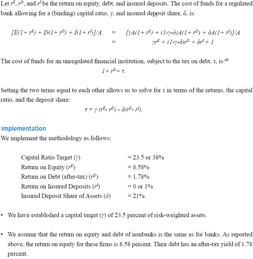
Calculating the Leverage Tax.

The leverage tax calculation takes the following form:

Endnotes

40 The IMF database reports 28 OECD crises over the period from 1970 to 2011. These crises represent 24 countries. Thus, we measure the probability as 28 crises divided by 1008 country-years.

41 The $7.684 trillion and $4.578 trillion numbers are aggregated Y-9C values for the targeted banks as of year-end 2015. Returns are also measured as of year-end 2015.

42 To calculate the GDP effect, we feed a 51-basis-point reduction in spreads into the FRB/US model, which will cause an increase in the estimate of future GDP. The potential “improvement” in GDP is the number we present in Table 4.

43 See the model at https://www.federalreserve.gov/econresdata/frbus/us-models-about.htm.

44 FRB/US does not have an analytical steady state.

45 In particular, the monetary policy reaction function is
                 R_t = 0.85R_t-1 + 0.15(1.09 + π_t + 0.5(π_t  – 2) + x_t )
where R_t is the federal funds rate, π_t is four-quarter core PCE inflation, and x_t is the output gap. Using a non-inertial version of the rule yields a negligibly larger output effect.

46 Bianchi (2011) imposes the tax on the principal and interest paid on the debt. All debt is short term in his model. We choose to impose the tax on the principal alone to avoid any bias in favor of shorter-maturity debt that typically carries a lower interest rate.

47 In November 2016, deposit rates were very close to zero. Short-term interest rates have increased several times since then, but deposit rates remain sufficiently low as to not materially change our results. A 100-basis-point increase in the deposit rate results in a 21-basis-point increase in the tax rate. 

48 We assume, for this calculation, that shadow banks fund themselves entirely with debt; thus, the debt of the sector equals the assets of the sector. Relaxing that assumption, that is, allowing for shadow bank equity, would reduce the tax rate required to equalize funding costs.