Author


Income inequality is a topic of much research and heated debate—concern well warranted given the substantial and continuing rise in inequality over the past four decades. But income risk—intimately related and arguably of equal concern to workers, families and firms—has received far less attention. This essay seeks to redress that imbalance. It provides a close look at income risk, discussing findings from recent research that uses innovative technique and draws upon a wealth of new data.
Every person and each segment of the U.S. population experiences volatility in annual earnings; the changes from one period to the next may be trivial, but in some years they can also result in great hardship or tremendous opportunity. Losing a job, being promoted, suffering an illness or becoming disabled—all are often unforeseen events that dramatically affect income flows and economic opportunities for individuals, households and businesses. To the extent that policymakers and the public seek to reduce the harm (or enhance the prospects) that income volatility creates, they should include income risk in the broader discourse on income and wealth in the United States and abroad. The research reviewed here aims to contribute to that discussion.
Distribution versus uncertainty
To begin, it’s important to distinguish between inequality and risk. Income inequality measures how income levels are distributed from highest to lowest across a population at a given point in time: One individual may earn $35,000 in a year while another earns three times that. To the extent that workers can move across the income distribution—from lower to upper income levels, or the reverse—some of these differences will average out over time and may not have very large welfare consequences for the economy as a whole. Income mobility is itself an important, but distinct, concern.
Income risk measures a very different economic phenomenon: the uncertainty that individuals (or firms) experience because of income fluctuations. A household could find its annual income cut in half (or doubled) from one year to the next. Some of this variation is inescapable. As the economy goes from expansions to recessions, and as a person’s health declines with age, incomes tend to fall. These are inevitable phenomena, but their timing is uncertain, leading to substantial insecurity.
Income risk also captures many labor market events that cause major hardship—job losses, demotions, jobs disappearing due to factory closures, employer bankruptcies, industry declines and so on. Even in an economy where inequality is not rising or is fairly modest, the magnitude, unpredictability and degree of insurability of income fluctuations can have a life-changing impact on workers and their households.
Understanding income risk with better data and stronger tools
Despite its importance in daily life and over entire lifetimes, the nature of income risk is not well understood. This is due in part to a relative dearth of high-quality “panel” data sets on individual earnings. A panel data set tracks the path of the same individuals (or households, businesses, states, countries and the like) over time; these data measure the relevant statistic of the same units at regular intervals for a long stretch of time and for many individuals. For a variety of reasons—small samples, attrition over time, nonrandom and unrepresentative selection, measurement or reporting errors—good panel data are often hard to come by. Income inequality, by contrast, can be measured with “cross-sectional” data, which are generally easier to gather and therefore more plentiful.
Poor data quality forces researchers to make strong restrictions and statistical assumptions that may be unfounded, and this combination of data issues and necessary restrictions on methodology has yielded a wide range of conflicting answers to questions about income risk. My earlier research on these topics relied on these small data sets and imperfect methods, making me increasingly uncomfortable about their use and motivating me to seek out better data and improved technique.
Fortunately, a number of newly available data sets have allowed economists, myself included, to explore trends and patterns in income risk in more detail with fewer assumptions than required with earlier data sets. This has yielded new and often surprising insights.1
In this essay, I discuss new research findings on three dimensions of income risk: Changes over (1) the business cycle (that is, during recessions and expansions), (2) the life cycle and (3) the long run—for example, over the past 40 or so years.
Individual income risk over the business cycle
What happens to individual income risk in recessions? Can the fortunes of a worker during a recession be predicted by a characteristic observed and measured prior to the recession? Answers to these questions can deepen society’s understanding of income risk.
How does income risk change during recessions and expansions?
The conventional wisdom among economists has long been that income shocks become much larger in recessions, resulting in much higher income risk. Economists believed that this was reflected by a rise in the statistical variance of income shocks—that is, variance is “countercyclical.”2
Although the hypothesis of countercyclical variance is consistent with the plausible idea that many individuals experience large negative shocks in recessions, it also implies (perhaps less plausibly) that, with a larger variance, many more individuals experience larger positive shocks in recessions than in expansions.
Serdar Ozkan, Jae Song and I (2014) have recently revisited these conclusions, using new and deeper data that allow us to make fewer assumptions—that is, we don’t have to rule out statistical variations and possibilities simply because data limitations require it. With better data and stronger econometric tools, we reach some unexpected conclusions.
Using data from the Social Security Administration (SSA) on tens of millions of U.S. workers, my co-authors and I document two new findings on the cyclicality of income risk. First, the variance of income shocks is not countercyclical. Contrary to conventional wisdom, it does not rise (or fall) in recessions; in fact, the dispersion of income shocks hardly changes at all over the business cycle.
Figure 1 shows this clearly, plotting the standard deviation (a measure of variation) of one-year income changes (proxies for income shocks) from 1978 to 2011. (The gray areas designate recessions, as determined by the National Bureau of Economic Research.) The variance of individual income changes is largely stable during recessions and expansions, though slightly declining over the entire time span.
At first blush, this seems a bit surprising; casual observation tells us that income risk seems higher in recessions. Indeed, this informal impression is quite correct, statistically. The answer to the apparent paradox lies in the fact that there is more to risk than variance alone.
Another crucial aspect of income shocks, also closely tied to what we commonly think of as risk, is their asymmetry: how likely large negative shocks are relative to large positive shocks. This asymmetry is measured by a statistic called skewness, and our empirical analysis reveals that the skewness of income shocks is strongly procyclical. That is, during recessions, the upper end of the shock distribution collapses: Large upward income changes become less likely. Simultaneously, the bottom end of the distribution expands: Large drops in income become more likely.
With this understanding of both variance and skewness, we therefore arrive at a more nuanced picture of income risk during recessions and expansions. While the dispersion (variance) of shocks does not increase during recessions, as previously thought, shocks become more left skewed and, hence, more risky during recessions.
This can be seen in Figure 2, which plots skewness for one-year income changes. Each point reflects income change from that year to the year after, and with the exception of the early 1990s recession, the line falls right before a recession begins and recovers near the end of the recession. The figure thus shows that skewness is substantially more negative in recessions, meaning downside risk increases in recessions and upside moves become more likely in expansions.
Can individual income risk be predicted?
A second question we ask in this paper (Guvenen, Ozkan and Song 2014), and one that has received little attention in previous work, is whether the fortunes of a worker during a recession can be foreseen by an observable characteristic measured prior to the recession. If so, this would imply that business cycle risk has a predictable component. Most previous research has suggested that income risk is purely idiosyncratic and largely unpredictable.
By developing what economists call a “factor structure,” whereby an aggregate shock can be seen to have dissimilar effects on workers with differing characteristics, scholars can better understand who is most at risk during recessions and can thereby better design policies to address that risk.
We found that one variable in particular, the average earnings of a worker over the five-year period that precedes a recession, strongly predicts how much that worker will suffer during the recession: Lower prerecession earnings predict larger subsequent losses.
Figure 3 plots this relationship, showing income changes over all recessions since 1978. The horizontal axis shows percentiles of the five-year average income distribution for individuals in the economy immediately before a recession begins; the vertical axis shows average income change during the given recession. As seen, the pattern is very strong during recessions: an upward-sloping, nearly straight line for workers who enter the recession with incomes between the 10th percentile and the 90th percentile of the income distribution.
A few concrete examples from particular episodes clarify the relationship. Workers with incomes at the 10th percentile before the Great Recession suffered an average earnings loss 18 percentage points larger than those at the 90th percentile. The 1980-83 double-dip recession had just as strong an impact, hitting those with lower prior earnings harder than those at higher levels. The two smaller postwar recessions exhibit the same relationship, but smaller differential between recessionary impact on lower and higher earnings percentiles.
This pattern reverses itself for very top earners; they lose more during recessions than workers with slightly lower prerecession incomes. And the income loss for top earners was much larger: Workers in the top 1 percent before the Great Recession lost on average 30 percent of their income between 2007 and 2009. Those in the top 0.1 percent lost 50 percent of their prerecession income between 2006 and 2011 (a longer period that covers many years after the end of the recession).
Surprisingly, the Great Recession was not the most severe recession for very top earners: Earnings losses for the top 1 percent and 0.1 percent were more severe during the 2000-01 recession and just as bad during the 1989-94 period. A caveat: These data are on labor earnings and so do not include capital income, but they do include bonuses, restricted stock units at time of vesting and exercised stock options.
Turning to economic booms, it is clear from Figure 4 that a more complex pattern is at work when the economy prospers. In particular, since 1978, workers who entered an expansion above the 70th percentile of the income distribution enjoyed earnings gains that rose with prior-income percentile; that is, those at the 75th percentile, prerecession, gained more than those at the 70th, but gained less than those at the 80th and so on. This stretches the income distribution at the top end, meaning that the richer got still richer than those slightly less rich.
The opposite happens at the lower end, where those with lower pre-expansion income see larger increases in their income during the subsequent expansion than those with somewhat higher preboom incomes, allowing them to catch up to the rest of the workers. This catching-up phenomenon was very strong during the 1990s expansion, but relatively weak during the other two expansions.
The relationships we document here have an important implication for the well-documented fact that income inequality rises during recessions. Our results show that this rise in inequality is due in large part to the upward-sloping factor structure during recessions and its reversal during expansions. That is, those who enter a recession with a lower income experience larger losses during the recession than those who enter with a higher income, and during expansions, those with higher pre-expansion incomes experience smaller gains than those with lower earnings. From the bottom percentiles toward the top (left to right), the lines in Figure 4 slope down (below the 70th percentile) and the lines in Figure 3 slope up (below the 90th percentile). This contrasts with the conventional wisdom mentioned earlier that inequality rises because the dispersion of income shocks increases in recessions, for which we find no evidence.
Other nations, households and social insurance
The analysis in the preceding paper (Guvenen, Ozkan and Song 2014) raises three questions.
-
Are the business cycle patterns (the flat variance and the procyclical skewness of individual income) unique to the United States, or do they hold in other developed economies?
-
Do these findings for individual male earners extend to household earnings, which might benefit from within-household insurance—that is, two-earner households?
-
How are these patterns affected by government social insurance policies in the form of unemployment benefits, the welfare system and the tax system?
To provide a broad perspective on these questions, my paper with Christopher Busch, David Domeij and Rocio Madeira (2015) studies individual- and household-level data from Germany and Sweden covering roughly the same time period as the first paper. We supplement these with U.S. data from the Panel Study of Income Dynamics, a survey-based panel data set. These data sets provide information not only on household income, but also on taxes and a broad range of government benefits.
The answer to the first question—applicability to other nations—is that the cyclical behavior of both individual and household income is remarkably similar in all three countries: flat variance and procyclical skewness. Given how different these national labor markets are, this similarity is somewhat surprising. Furthermore, skewness is procyclical within almost every subgroup—education, gender, type of employment, occupation and so on—that we examined. The fundamental forces driving skewness over the cycle seem to be a robust feature of developed economies.
Second, moving from individual earnings to household earnings makes only a small difference to cyclicality of risk, suggesting that there is little within-household insurance against the business cycle component of individual income risk. That is to say, households with two or more earners are not better able to withstand recession risk than are those with a sole provider.
Third, government-provided insurance plays a more important role (than intrahousehold insurance) in reducing downside risk in all three countries; their effectiveness is weakest in the United States and is much stronger in Germany and Sweden, which have policies of comparable effectiveness.
Life-cycle risk, long-term risk and big data
How does income risk change over time spans longer than business cycles, in particular, over the life cycle? What age and income groups receive shocks that are more difficult to insure? These questions lie at the heart of many government policies, but they are hard to answer conclusively for the same data and statistical reasons discussed previously. In fact, the data problems are more acute in this context precisely because answering such questions requires subdividing the data by age and income groups, leading to very small samples and imprecise estimates. To analyze small samples, statisticians have to make strong assumptions that may or may not be valid.
One of the most common assumptions is that the statistical values (for income, say) of the entire population follow a “normal” distribution—that is, a symmetrical bell-curve pattern. This familiar pattern is methodologically simple to analyze, and making the assumption becomes very convenient when samples are small. But the reality is often different; many statistics don’t fall into the familiar bell curve, and analyzing them as if they do leads to false conclusions.
The best way around this obstacle is much bigger samples and, fortunately, the massive statistical sets from SSA databases provide exactly that. Fatih Karahan, Serdar Ozkan, Jae Song and I (2015) take advantage of this invaluable resource to revisit key questions about the nature of earnings dynamics over the life cycle.
Income changes don’t follow a bell-curve distribution
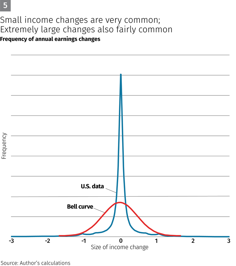
One of our main findings is that the distribution of both annual and longer-term income changes is far from “normal.”3 Very small income changes are much more common in actual U.S. data than in the ideal normal distribution, middling shocks are relatively rare and extremely large shocks are experienced far more often than a bell curve would have us believe.
This feature of a distribution is called “excess kurtosis”—kurtosis meaning how flat or sharp the peak of a distribution curve is. The earnings change data are “leptokurtic,” denoting that the curve is very sharply pointed compared with a bell curve: Small income changes—close to zero—are very common. Figure 5 shows this in that the blue curve for U.S. income change data peaks sharply while the red line, a bell curve, shows a relatively mild bulge.
While leptokurtic is an intimidating term, its reality when applied to income changes is easy to understand. Most workers stay at their jobs year to year, and their income usually doesn’t change dramatically from one year to the next—it might rise at the rate of inflation or with a small raise; it could decline if the annual bonus shrinks. Every once in a while, though, something big happens: A worker might suffer a serious illness or be disabled; a factory could shut down. Such unfortunate events—though rare—would lead to major negative income shocks. Conversely, a worker could be blessed with a big promotion or a job change with a considerably higher salary. Again, exceptional circumstances, but big (positive) income shocks. That, in a nutshell, is leptokurtic.
To give some magnitudes, a normal distribution (with the same mean and variance as in the U.S. data) would predict that only 8 percent of individuals experience an annual earnings change smaller than 5 percent (either negative or positive); the actual U.S. data show that 35 percent experience these near-zero changes. The probability that a worker will receive a very large shock (a fivefold increase or an 80 percent drop) is eight to 12 times higher in the data than under normality.
A second important deviation from normality is that the distribution of earnings shocks is not symmetric: It displays large negative skewness. That is to say, large downward movements in earnings (what could be thought of as disaster shocks) are more likely than large upward swings. This asymmetry is seen in Figure 6, where the blue line denoting actual U.S. data skews to the left compared with the symmetrical bell curve (red line).
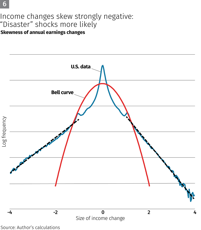
Third, the extent of both deviations from normality changes substantially with the individual’s age and income level. In particular, kurtosis and negative skewness are modest at age 25 and at low income levels, but they both become more extreme (higher kurtosis and more negative skewness) as individuals get older—up to about age 55—and/or their income levels rise up to about the 80th to 90th percentile. Then both patterns reverse at older ages and highest income levels.
Again, this statistical description sounds dry as it abstracts from daily experience, but it is easily translated into everyday language. As workers remain at the same job for many years, they tend to reach salary caps and exhaust opportunities to move up. That puts a negative skew on income changes, as does the fact that their downside risks tend to increase, from negative health shocks or their skill sets being overtaken by technological advances.
What do these deviations from normality mean for analyses of individual income risk? We find that even in the presence of ample income-smoothing opportunities—from household borrowing and saving, government welfare programs and progressive income taxes for redistribution—the welfare costs of the remaining fluctuations are very large, on the order of 25 percent to 40 percent of consumption per household per year. This is about two to three times larger than a normal (bell-curve) distribution would predict.
Recent follow-up work has re-examined a wide range of economic questions in light of these new findings on the nature of income risk. Economists are using models that incorporate negative skewness and excess kurtosis to predict asset prices, to estimate tax policies that optimize marginal tax rates for top labor earners and to better understand the mechanisms that transmit monetary policy to the macroeconomy.4
Summary, future work and conclusion
The use of newly available data sets has upended some previously held beliefs about the nature of income risk. Economists have long assumed that the variance of income shocks was procyclical, but recent research finds this variance to be very stable during both recessions and expansions (and for nearly all subpopulations of workers). However, research does find that skewness of income shocks is strongly procyclical. So during recessions, the dispersion of shocks doesn’t increase, but income shocks become more left-skewed and hence more risky.
Research with new data sets also finds that one characteristic is very useful in predicting the impact of a recession on an individual worker’s income: his or her income in the five years prior to the recession. Those with higher prerecession incomes suffer less than those at lower previous income levels. This relationship doesn’t hold as strongly during expansions, however; the pattern is more complex. Over all, this indicates that the recessionary rise in income inequality is due in large part not to larger income shocks, but to this differential and predictable impact of prerecession income levels.
Recent research also finds that these patterns hold in other advanced economies, like Germany and Sweden, despite their dissimilar labor markets. We find on the one hand that households with more than one income earner are no better able to withstand income risk than those with just one earner. On the other hand, government policies to mitigate downside risk are effective, more so in Germany and Sweden than in the United States.
We’ve also discovered that the distribution of both annual and longer-term income changes is far from normal, as long assumed. Near-zero income changes are far more common than a normal distribution suggests, middling shocks are rare and extremely large shocks are experienced far more often than thought. Moreover, such shocks are not symmetric: Large downward movements in earning are much more likely than large upward swings. The extent of such deviations from a normal distribution varies by age and income level, and we find that despite the presence of progressive taxation, government welfare programs and household borrowing and saving, income fluctuations and their welfare costs are extremely large, implying a role for even more generous government policies.
In addition, in a new research project with Nicholas Bloom, Luigi Pistaferri, John Sabelhaus, Jae Song and Sergio Salgado (2017), we turn from business cycle fluctuations to long-term trends and explore the downward trend in income volatility seen in Figure 1. Specifically, we show that individual income growth has become less and less volatile since the 1980s, and this fact is robust across gender and age groups, within industries, for individuals who work for large or small firms or for young or established firms and for workers who stay at their job as well for those who switch jobs.
This finding contrasts with the conventional wisdom among economists that income volatility has been trending up during the same period (interpreted as increasing risk or uncertainty). This earlier work was predominantly based on two survey data sets, and we also provide some explanations for why those survey data led to that conclusion.
A key contribution of this new project is to link patterns of income volatility on the worker side to outcomes (and volatility) on the firm/employer side. Using the information revealed by these linkages, we investigate several potential drivers of this trend to understand if declining volatility represents a broadly positive development—declining income risk and uncertainty—or a negative one, that is, declining business dynamism.
In just a few years, research into income risk has revealed many new findings that go against the conventional wisdom of even five years ago, and the future is likely to yield still more. The use of big data has allowed scholars to escape the confines of strong assumptions and restricted models, and enabled us to begin to understand risk with all its complexity, depth and nuance.
Endnotes
1 One data set used in this research comes from the Master Earnings File of the U.S. Social Security Administration. The MEF covers the entire U.S. population with a Social Security number from 1978 to (at present) 2013. For every individual, it contains data on labor earnings (wage income from W-2 forms and self-employment income from Schedule SE), as well as some key demographic variables and employer identifiers.
The substantial sample size (600 million individual-year observations in a 10 percent subsample) allows us to employ fully nonparametric methods and take what amounts to high-resolution pictures of individual earnings histories. (“Parametric” methods make assumptions about the properties of the distribution of the population whose data are being analyzed—the standard assumption is a normal, or bell curve, distribution. With “nonparametric” methods, we don’t need to make any such assumptions.)
2 By “variance” I mean, informally, how much the high and low values of the data set differ from the data set’s statistical mean. “Countercyclical” in this context means that when the economy declines, variance rises, and vice versa.
3 Technically, the income changes and distribution normality as analyzed and discussed here are logarithms of these statistics.
4 For specifics, see Constantinides and Ghosh (2014) for research showing that an incomplete markets asset-pricing model with countercyclical (negative) skewness shocks generates plausible asset pricing implications. See also Schmidt (2014), who goes one step further and considers both negative skewness and thick tails (targeting the moments documented in my work with Ozkan and Song 2014) and finds that the resulting model also provides credible asset price predictions. Turning to fiscal policy, Golosov, Troshkin and Tsyvinski (2014) show that using an earnings process with negative skewness and excess kurtosis implies a marginal tax rate on labor earnings for top earners that is substantially higher than under a traditional calibration with Gaussian (normal) shocks with the same variance. Finally, Kaplan, Moll and Violante (2016) show that introducing earnings shocks with excess kurtosis into a New Keynesian model with household heterogeneity has important implications for the monetary transmission mechanism.
References
Bloom, Nicholas, Fatih Guvenen, Luigi Pistaferri, John Sabelhaus, Jae Song and Sergio Salgado. 2017. Why Has U.S. Earnings Volatility Been Declining for Four Decades? Working paper.
Busch, Christopher, David Domeij, Fatih Guvenen and Rocio Madeira. 2015. “Higher-Order Income Risk and Social Insurance Policy Over the Business Cycle.” Working paper, University of Minnesota.
Constantinides, George M., and Anisha Ghosh. 2014. “Asset Pricing with Countercyclical Household Consumption Risk.” Working paper, University of Chicago.
Golosov, Michael, Maxim Troshkin and Aleh Tsyvinski. 2014. “Redistribution and Social Insurance.” Working paper, Princeton University.
Guvenen, Fatih, Fatih Karahan, Serdar Ozkan and Jae Song. 2015. “What Do Data on Millions of U.S. Workers Reveal about Life-Cycle Earnings Risk?” Working Paper 20913, National Bureau of Economic Research.
Guvenen, Fatih, Serdar Ozkan and Jae Song. 2014. “The Nature of Countercyclical Income Risk.” Journal of Political Economy 122 (3): 621-66.
Kaplan, Greg, Benjamin Moll and Giovanni L. Violante. 2016. “Monetary Policy According to HANK.” Working Paper 21897, National Bureau of Economic Research.
Schmidt, Lawrence. 2014. “Climbing and Falling Off the Ladder: Asset Pricing Implications of Labor Market Event Risk.” 2014. Working paper, University of California at San Diego.