Like criminals themselves, crime data are both plentiful and elusive, and it doesn’t take long to get buried under the available numbers. The Bureau of Justice Statistics, the Federal Bureau of Investigation, and various state and local agencies churn out reams of information about criminal activity and the criminal justice system on an annual basis, some of it available online, much of it incompatible or incomplete across agencies or jurisdictions.

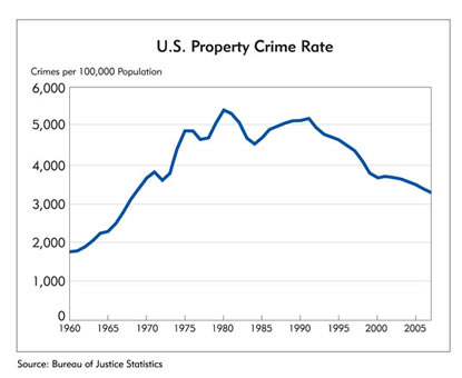
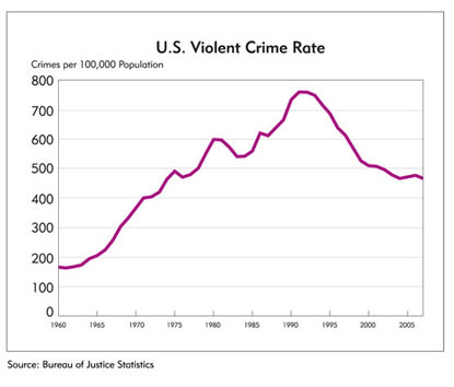
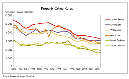
Graphs of crime rates in the United States look like mountains; the good news is that, generally speaking, the country is headed down from the summit. Violent crimes peaked in 1991 and have dropped ever since, though recent declines have been modest compared with those seen during the 1990s. The nation now experiences about 465 violent crimes per 100,000 population, a level last seen in the mid-1970s. Property crimes climbed steadily from 1960 to 1980, topping out at about 5,300 per 100,000 population. Rates declined until mid-decade and climbed again until 1991; property crimes have dropped ever since, reaching about 3,200 in 2007, a level last seen in 1969.
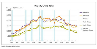
Among district states, property crime rates have followed a very similar trend, but two states, North Dakota and South Dakota, have enjoyed much lower levels of crime, with the Dakotas’ property crime peaks (around 3,000 in 1980) barely exceeding the current troughs of other district states and the nation as a whole. Currently, South Dakota’s property crime level is about half the national level and North Dakota’s is a bit higher; these rates are the lowest in the nation (see map). Minnesota, Montana and Wisconsin property crime rates are all at about 90 percent of U.S levels.
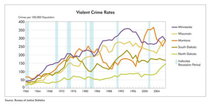
Violent crime in the district is a different animal. Montana had an initial violent crime crest in the early 1980s, then a decline until the late 1990s, when reported violent crime rates soared for six years, reaching a peak in 2003. The violent crime rate has declined since then, down from 365 per 100,000 to 288 in 2007. South Dakota’s rate experienced a similar early crest in the mid 1970s, then dropped until the late 1980s and climbed to a second peak in 1994, whereupon rates dropped and leveled off at about 170. Minnesota and Wisconsin have had parallel paths in violent crime, by and large, with peaks in the early 1990s, a bit after the national peak, and then trending downward, though both have had increases in recent years. North Dakota has the lowest level of violent crime in the district, and the nation, remaining well below 100 per 100,000 until 2005, when it jumped to 111. In 2007, the rate was 142, well above the North Dakota average, but still less than half the rates experienced in Minnesota, Montana and Wisconsin, and less than a third the national rate.
Some explaining to do
So, what accounts for these different rates of crime, across states and over time? Does economics play a role? And specifically, are economic recessions associated with increases in crime? First, a look at recessions.
In the charts of violent and property crime rates, shaded blue columns represent years in which the National Bureau of Economic Research, the nation’s arbiter of recessions, declared that a recession took place. The most acute eye would have a difficult time discerning any consistent relationship between those recessionary years and specific trends in crime. During the difficult 1974 recession, property crime rates were climbing, but during the hard recession of 1981–82, they dropped substantially.
A numerical comparison of crime rates might better gauge the relationship. And indeed, from 1960 to 2007, the average property crime rate in the United States was 19 percent higher during recession years than during nonrecession years. In district states, as well, this relationship held. Wisconsin’s average recession year had a property crime rate of 3,826, about 24 percent higher than its average nonrecession year.
In recent years, though, this trend has been weaker. In the period 1980–2007, recession years had an average property crime rate 14 percent higher than nonrecession years in the United States, and just 10 percent higher in Montana and North Dakota.
Curiously, the association is reversed or largely absent for violent crime. With the exception of Montana and the United States, district states had lower or about the same level of violent crime in recessionary years. This was especially true for the 1980–2007 period.
This apparent association between higher property crime and recession is suggestive, certainly. But it’s far from a compelling correlation, let alone causal proof, because it relies on relatively few observations of recession years, just seven in a 48-year span, most of which occurred during the peak crime eras of the early 1980s and 1990s. The trends that led to those peaks were in place well before recession hit.
Correlations
Perhaps an analysis of year-to-year correlations between crime rates and possible causal factors could provide richer context based on more observations. The FBI cites 13 categories of factors “known to affect the volume and type of crime occurring from place to place,” ranging from population density and climate to modes of transportation, and each of the categories includes a multitude of variables. “Economic conditions, including median income, poverty and job availability,” is just one of the 13.
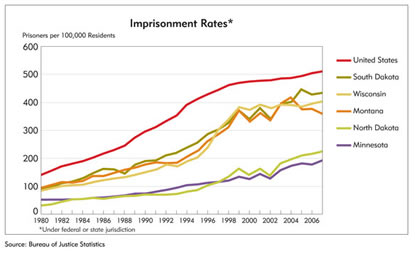
Of course, economists, in their crime models, generally put economic variables at center stage; these may include unemployment rates, personal income levels, poverty rates, measures of inequality and wage levels. Often they’ll also include variables reflecting legal disincentives to engage in crime. So, for example, the imprisonment rate—number of people held in prison per 100,000 residents—may be part of the model, since it can measure both a potential criminal’s sense of probability that he or she will be caught and punished and the level of a government’s incapacitation of likely criminals: If they’re in jail, they can’t rob banks.
Economists have also looked at factors as varied as indexes of consumer sentiment and legislation to permit abortion, to allow the carrying of concealed weapons or to prohibit lead in paint. Demographic information, such as the percentage of total population in a prime crime category of, say, males 15-24 years old, is also frequently included.
As discussed in the cover article (see “The mystery of crime”), empirical studies conducted in the four decades since Gary Becker first elaborated his economic model of crime have proven surprisingly inconclusive. Still, it may be interesting to explore some of the relationships at work in the Ninth District.
To understand crime correlations in the Ninth District, data for the United States and five district states (including all of Wisconsin, but not Michigan) were collected for each year from 1980 to 2007 on eight variables: the index of consumer sentiment, poverty rates, income inequality (Gini coefficient estimates), per capita personal income, unemployment rates, imprisonment rates and percentage of population composed of males between 15 and 24 years old, plus property crime rates.
Of these, the correlations between crime and consumer sentiment, poverty, unemployment and young male population were weak or inconsistent across states—a surprising finding given that a number of empirical studies have suggested connections. Perhaps different relationships explain crime in the Upper Midwest.
On the other hand, consistently strong negative correlations were found between crime and inequality, per capita income and the imprisonment rate. That the crime correlation for inequality was negative is surprising, given some research indicating a positive relationship between inequality and crime, but an even stronger correlation between per capita income and inequality rates may provide a partial explanation.
The negative imprisonment/property crime correlation was one of the strongest relationships, but the direction of causality is open to question (see charts below). Perhaps putting people in jail prevents crime, but it could also be that higher levels of crime lead to higher levels of arrest and sentencing.
Regression to the mean streets
One weakness of correlation analysis is precisely that direction of causality is hard to ascertain, but another is that a simple correlation between two variables may obscure the influence of a third variable. Crime may be negatively correlated with imprisonment, for instance, and positively correlated with unemployment, but simple correlation analysis can’t measure the independent strength of each relationship. That calls for a different statistical technique: multiple regression analysis, a method that allows the analyst to mathematically measure the individual influence of a single “explanatory” variable while holding other variables constant.
To better explain the statistical relationships between crime rates in the Ninth District and several possible explanatory variables, county-level data were gathered on several factors potentially related to crime, and a regression analysis was done. The results are informative, but they’re by no means definitive. There are several reasons to read these results with caution.
First, though theory provides some guide to interpretation, even regression analysis doesn’t prove causality—it simply gives a richer understanding of the correlations between variables. Regressions are more sophisticated than simple correlations, but they don’t prove causality. Second, the data are incomplete and possibly inaccurate. Crime rates, as mentioned elsewhere in these articles, are especially prone to inaccuracy. But even numbers of police officers in any given county in a particular year may be mistakenly recorded.
Third, regression analysis is prone to a number of statistical shortfalls. Economists use a variety of advanced techniques in an attempt to address these shortfalls, but even then other complications (and debates) arise. This article reports the results using a fairly standard statistical procedure, a “fixed-effects” model.
A fixed-effects model has been chosen with the assumption that whatever the influence of the included variables, other unobserved and omitted characteristics inherent to each district state will affect crime rates—things like legal and political structures that are important to the level of crime and relatively consistent (or “fixed”) over time within each state. Those state-by-state effects are included in the statistical model along with the more traditional explanatory variables. The model used here also accounted for these fixed effects at the county level.
Getting a fix
In this fixed-effects regression, the fedgazette seeks to explain the variation of one dependent variable (property crime rate) with several independent variables: per capita personal income, unemployment rates, number of police officers per capita, clearance rates, population, percentage of population between 14 and 24 years old and per capita government expenditure on education. But again, caution is needed in interpreting results: Regressions describe statistical associations, not causal mechanisms.
Economic theory suggests that unemployment rates will be positively related to crime rates, other things equal, because fewer legitimate job offers should make criminal activity more attractive. For similar reasons, per capita income should be negatively related to crime rates—if people have higher incomes, they should find illegal activity less appealing. Theory also suggests that higher numbers of police and higher clearance rates will be negatively related to crime rates, because both represent higher costs (probabilities of being caught and charged) of crime. Because young people, particularly young men, are more likely to commit crime than other population groups, a higher fraction of them is likely to be positively related to crime rates. Per capita government expenditures on education were included as a variable representing public efforts to provide better options for youth; higher levels of expenditure, other things equal, may be inversely related to crime rates.
There are 303 counties in the district, including the upper Peninsula of Michigan, but because accurate, consistent data weren’t available for them all, 14 were dropped from the analysis. Data were gathered on crime rates and other variables from 1990 to 2006. Ultimately, then, the analysis examines 17 years of data for about 289 counties, seeking to clarify their interrelationhips over time and across counties.
Here’s what the regression found
Income and population: Initially, it appeared that per capita income had a strong positive link to crime, other variables held constant. But when population was also included in the regression equation, income lost its statistical significance, while population retained significance, suggesting that—as seems intuitive—highly populated counties will have higher crime rates, regardless of their income levels.
Unemployment: As predicted by theory, higher unemployment rates were associated with higher crime rates in district counties. But the quantitative importance of this variable (and even its statistical significance) was very small, meaning that changes in unemployment didn’t have much explanatory power. This finding is consistent with the conclusions of most other empirical studies on the matter.
Police officers: The number of police officers had little or no statistical relationship to crime rates when other variables were taken into account. Economic theory suggests that more police should represent more deterrence and therefore less crime, but politics suggests that police numbers may rise when crime is prevalent. The findings here suggest a balance of the two.
Clearance rates: In this study, clearance rates are calculated as a ratio of the number of arrests to the number of offenses. While not a perfect measure of what police consider a clearance rate, the variable was strongly associated with crime, in a negative direction, meaning that higher rates of arrests-to-offenses were associated with lower crime rates, other things equal—a finding supportive of the deterrence hypothesis.
Youth: Higher percentages of youth-to-population were positively associated with crime rates, a demographic relationship found consistently in most crime research.
Education spending: More government spending on education was negatively linked to crime rates, holding constant other factors, suggesting that efforts to build human capital might provide positive alternatives to illegitimate activity.
State fixed effects: Once other characteristics were held constant, crime rates in the Upper Peninsula of Michigan and both Dakotas were lower than in Minnesota, while in Wisconsin’s district counties, crime was higher. The fixed effect for Montana wasn’t significantly different from zero.
What it all means
Again, because of the statistical and data problems described above, these findings should be viewed as very tentative. They are, nonetheless, generally in line with conclusions from other empirical research: Unemployment rates are positively related to crime, but they don’t seem to have much explanatory power. Numbers of police per capita had no apparent association, but clearance rates did. More crime was likely in counties with higher fractions of young people. Spending on education was negatively linked with crime, indicating that schooling may reduce the relative appeal of crime. Does this mean that crime is no longer a mystery, that it’s possible to know whether or not a recession will result in more crime in the district? Far from it.
Statistical analysis clarifies links among variables, but it doesn’t prove causation or give powers of prediction. This brief analysis has barely scratched the surface of a problem as old as humanity itself.
Terry Fitzgerald, senior economist; Rob Grunewald, associate economist; and Clint Pecenka, research assistant, contributed to this article.


