In “Financial Frictions and Fluctuations in Volatility,” a Minneapolis Fed staff report published in July, economists Cristina Arellano and Patrick Kehoe of the Minneapolis Fed and Yan Bai of the University of Rochester develop a model that can convincingly generate several central macroeconomic patterns seen in U.S. data during the Great Recession. In particular, the economists explore the financial and microeconomic underpinnings of sharp declines in employment and economic output between 2007 and 2009, accompanied by relatively stable labor productivity. In almost all recessions, productivity and output both decline, but in the most recent downturn, productivity was nearly unchanged. What economic mechanisms account for this anomaly?
One clue that informs their investigation is the severe credit contraction during the recent U.S. financial crisis. Another clue, at the micro level, is the large increase in dispersion of growth rates among firms—that is to say, growth at some companies suffered very little during the crisis, while other firms contracted dramatically. Even during normal times, companies grow at different rates, of course, but during the 2007-09 recession, the range between the highest and lowest growth rates nearly doubled.
These observations are building blocks for a quantitative model with heterogeneous firms (for which growth rates can differ) and financial frictions (meaning that credit markets don’t function smoothly). The economists’ goal is to create a model in which increasing volatility at the firm level leads to higher dispersion in firms’ growth rates along with declines in both aggregate labor and economic output, but stable labor productivity. Their aim, in short, is to better understand the U.S. economy during the recent recession by building a model that can replicate its behavior between 2007 and 2009.
Central to the model: Risk, and firms hedging against it by trimming financial obligations wherever feasible—specifically, by hiring fewer inputs. “They key idea in the model,” write the economists, “is that hiring inputs to produce output is a risky endeavor.”
Firms receive revenue from selling their output only after they have already paid for inputs, such as employees, necessary to produce that output. Hiring labor (or buying materials or purchasing machinery) therefore entails risk, since demand for a firm’s output may fall after the input expenditure is incurred. If financial markets were “complete,” as economists say, firms could protect themselves against that event by borrowing against future profits; but in this model, financial market frictions mean that firms must bear the risk themselves.
“This risk has real consequences if, when firms cannot meet their financial obligations, they must experience a costly default,” observe the economists. “In such an environment, an increase in uncertainty arising from an increase in the volatility of idiosyncratic shocks leads firms to pull back on their hiring of inputs.” (Though the word “hiring” suggests employees only, here it applies to other inputs as well: raw materials, capital equipment and the like.)
If we build it, will it work?
The economists proceed in stages. First, they build a “benchmark” model. Then they calibrate and quantify it to gauge how well it matches real U.S. data. They create two alternatives to their benchmark model to pinpoint whether the results are driven by both factors (imperfect financial markets and volatility shocks) or just one. Lastly, they extend their model with refinements that bring it closer to how economists believe economies truly work.
The model has three key pieces:
- Firms hire inputs before knowing how much demand they’ll experience for their output.
- Financial markets don’t necessarily provide firms with credit, and they’re especially averse when the economy is volatile; as a result, firms default if they’re unable to pay their debts.
- Since firms pay a fixed cost to start their operations, they make positive profits in the future to cover those fixed costs; the cost of default is the loss of future expected profits.
These three essential parts mean that firms trade off expected risk and return whenever they choose their inputs. Hiring more inputs enables them to make more profit as long as they don’t default. But because more hiring raises their financial obligations, it also increases the chance of defaulting. It’s a tough choice, and becomes more so when the broader economy is looking uncertain—or, in the idiom of economics, “when the variance of idiosyncratic shocks increases.”
The model includes identical households, heterogeneous firms and financial intermediaries. Households buy goods produced by firms, but the demand for each good is subject to idiosyncratic demand shocks. The volatility of these demand shocks varies over time, and this is the source of aggregate fluctuations in the model.
Firms are the guinea pigs in this model. They differ from one another, and they face not only volatile demand for their products, but imperfect or incomplete financial markets that don’t allow them to insure against fluctuations in that demand. Thus, they may sink or swim based in large part on those fluctuations, as well as their hiring decisions. If they default on their debts, they fail: They “exit the market.”
Benchmark and beyond
The benchmark model is calibrated to the U.S. economy with standard values for such variables as interest rates, annual sales growth for firms and the like. The economists test the model with these parameters by checking whether it can match U.S. data accurately; it does—with, for example, the fraction of labor employed by new firms at 1.8 in both data and model, and the liability-to-sales ratio at 5.5 in the data versus 5.6 from the model. A near-perfect fit.
Then they see how it responds to “impulses”—that is, how the model’s mechanism reacts to a sudden increase in demand volatility. In this test, just as in the actual U.S. economy during the recent crisis, the model’s output and labor (that is, employment) drop strongly when volatility increases, but labor productivity (defined as the ratio of gross domestic product to aggregate employment) increases slightly at first and then stabilizes. “The overall response,” the economists write, referring to labor productivity, “is fairly flat compared to the responses of output and labor.”
In addition, wages fall about 1.4 percent after the volatility shock and then continue a slow decline, and the interest rate drops just a bit initially and remains slightly depressed. The benchmark, in short, works well as a representation of the U.S. economy during the financial crisis, at least for one-time shocks in demand volatility.
They then build two alternate versions of the benchmark to investigate whether this success is due primarily to its inclusion of incomplete financial markets or to its volatility shocks. This investigation finds that “both financial frictions and the source of the shocks—volatility instead of productivity—are critical to our benchmark model’s results” (emphasis added). In other words, neither financial frictions by themselves, nor just volatility shocks, are able to generate economic responses that resemble the real world during the Great Recession.
Real world testing
But the fundamental question is, how well can this model account not for a theoretical one-time volatility shock, but for a series of shocks like those experienced in the real economy during the Great Recession? The answer: very well. “We show that our model can account for much,” the economists write.
To reach that conclusion, they first find the volatility shock sequence that generates dispersion among firms’ sales growth rates similar to that actually measured in U.S. data between late 2007 and the third quarter of 2009. The data reveal nearly a doubling in this range of growth rates, from 17 percent to 31 percent. The economists feed that shock sequence into their model and see what happens to macroeconomic output, labor and productivity.
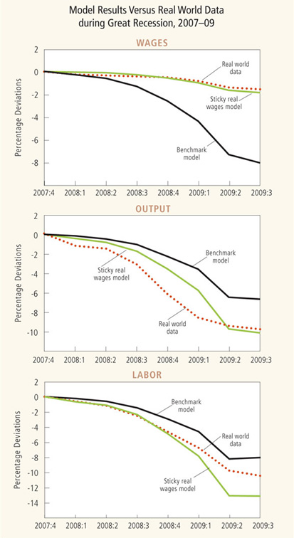
Given how crude the model is—in the sense of leaving out countless aspects of an actual national economy—it does a remarkable job of generating results similar to real world figures. “The model generates a decline in output of 6.5 percent, whereas in the data output declines 9.7 percent,” they find. And it “produces about an 8 percent decline in labor, whereas in the data labor declines about 10 percent.”
While not dead on, the model’s results are quite close, suggesting that the mechanisms at its heart are what drive the actual economy, through good times and bad. When the economists summarize the overall results, they conclude that the model “can explain 67 percent of the overall contraction of output and 73 percent of the contraction in labor during the Great Recession.” The model produces a fairly flat productivity profile for the recession, while in real data, productivity first falls and then rises modestly. But “both in the model and in the data, productivity at the end of this event is essentially unchanged … even though output has fallen 10 percent.”
Refinement
The economists explore several dimensions of, and refinements to, their model. One is to alter the model by introducing “sticky wages,” the idea that in the real world, most prices don’t change instantly. A gallon of gasoline may rise or fall in price several times a day or week, but wages, automobiles and even items on a restaurant menu take a while to adjust to trends in the economy—to a broad recession or to a rise in the cost of health care, steel or eggs. This factors into the model, since in the benchmark version of the model, wages fall when volatility increases, and such response dampens the labor adjustment firms make.
And indeed, by making the model’s input prices less responsive to volatility, the economists find that sticky prices “diminish offsetting equilibrium effects.” The charts on page 35 show their results. They compare real wage trends in the data, the benchmark model and the sticky real wage model for the entire span of the Great Recession and show that while they drop by about 2 percent in the data and over 8 percent in the benchmark model, “in the sticky real wage economy, real wages drop about the same as in the data.” Sticky real wages also amplify the output and employment effects of increased volatility.
Thus, Arellano, Bai and Kehoe’s model, with key features and additional enhancements, does a striking job of duplicating patterns seen in the U.S. economy in recent years. “Hence,” they conclude, “we think of the model as a promising parable for the Great Recession of 2007-2009.”


