Abstract (Note *)
Since the early 1990s, the United States has borrowed heavily from its trading partners. This paper presents an analysis of the impact of an end to this borrowing, an end that could occur suddenly or gradually.
Modeling U.S. borrowing as the result of what Bernanke (2005) calls a global saving glut—where foreigners sell goods and services to the United States but prefer purchasing U.S. assets to purchasing U.S. goods and services—we capture four key features of the United States and its position in the world economy over 1992–2012. In the model, as in the data: (1) the U.S. trade deficit first increases, then decreases; (2) the U.S. real exchange rate first appreciates, then depreciates; (3) the U.S. trade deficit is driven by a deficit in goods trade, with a steady U.S. surplus in service trade; and (4) the fraction of U.S labor dedicated to producing goods—agriculture, mining and manufacturing—falls throughout the period.
Using this model, we analyze two possible ends to the saving glut: an orderly, gradual rebalancing and a disorderly, sudden stop in foreign lending as occurred in Mexico in 1995–96. We find that a sudden stop would be very disruptive for the U.S. economy in the short term, particularly for the construction industry.
In the long term, however, a sudden stop would have a surprisingly small impact. As the U.S. trade deficit becomes a surplus, gradually or suddenly, employment in goods production will not return to its level in the early 1990s because much of this surplus will be trade in services and because much of the decline in employment in goods production has been, and will be, due to faster productivity growth in goods than in services.
The global saving glut
From 1992 to 2012, households and the government in the United States borrowed heavily from the rest of the world. As U.S. borrowing—measured as the current account deficit—grew, the U.S. net international investment position deteriorated by $4 trillion, and, by 2012, the United States owed the rest of the world $4.4 trillion. In this paper, we use a model developed by the authors (Kehoe, Ruhl and Steinberg 2013) that captures this increase in borrowing to study the different ways in which the United States can reverse its current account deficit and begin to pay down its accumulated debt. Our hypothesis for the driving force behind the United States’ borrowing is the global-saving-glut theory proposed by Ben Bernanke. In a March 2005 address, Bernanke (2005) asked,
“Why is the United States, with the world’s largest economy, borrowing heavily on international capital markets—rather than lending, as would seem more natural? … [O]ver the past decade a combination of diverse forces has created a significant increase in the global supply of saving—a global saving glut—which helps to explain both the increase in the U.S. current account deficit and the relatively low level of long-term real interest rates in the world today.”
The essence of the global-saving-glut theory is that increased saving in the rest of the world, primarily in China, resulted in foreigners purchasing U.S. assets rather than U.S. exports. As foreigners sold goods and services to the United States to finance these asset purchases, the price of these goods and services compared to those in the United States fell.
The balance-of-payments identity says that payments by U.S. residents to rest of the world (ROW) must equal payments by the rest of the world to U.S. residents:
ROW purchases of U.S. exports + ROW factor payments and transfers to U.S.
+ ROW purchases of U.S. assets
= U.S. purchases of ROW exports + U.S. factor payments and transfers to ROW
+ U.S. purchases of ROW assets.
This equation is an identity because accounting conventions make it hold at all times: An excess of payments made by the rest of the world over payments made by U.S. residents, for example, is counted as purchases of assets in the rest of the world by U.S. residents, that is, U.S. residents borrowing from foreigners. We can rearrange this identity as
(ROW purchases of U.S. exports − U.S. purchases of ROW exports)
+ (ROW factor payments and transfers to U.S. − U.S. factor payments and transfers to ROW)
= (U.S. purchases of ROW assets − ROW purchases of U.S. assets),
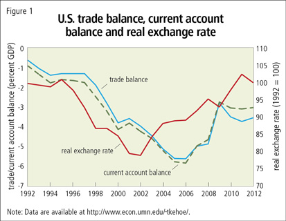
which says that the U.S. trade balance plus net factor payments and transfers from the rest of the world are equal to net U.S. asset accumulation in the rest of the world. The sum of the trade balance plus net factor payments and transfers from the rest of the world is referred to as the current account balance, which is also equal to net U.S. accumulation of foreign assets. The data in Figure 1 show that the U.S. current account balance is approximately equal to the U.S. trade balance because net factor payments and transfers from the rest of the world are small. Consequently, the balance-of-payments identity says that the trade deficit is approximately equal to foreign accumulation of U.S. assets.
Figure 1 also presents data on prices in the United States relative to those in the rest of the world, the real exchange rate between the U.S. dollar and a weighted geometric average of the currencies of its 20 most important trading partners. The real exchange rate between the U.S. dollar and the Chinese renminbi, whose principal unit is the yuan, for example, is
U.S.-China real exchange rate = U.S.-China nominal exchange rate x (Chinese CPI ÷ U.S. CPI),
where we measure the price level in each country using its consumer price index (CPI). To understand this real exchange rate, consider the units in which it is measured:
(dollars÷yuan) x ((yuan÷Chinese consumption basket) ÷ (dollars÷U.S. consumption basket)) = U.S. consumption basket ÷ Chinese consumption basket.
As the real exchange rate falls, fewer U.S. consumption baskets trade for one Chinese consumption basket, and the dollar appreciates.
Between 1992 and 2002, the real exchange rate between the U.S. dollar and the weighted sum of the currencies of its trading partners fell from 100 to 78.2. This means that prices of U.S. goods and services compared with those of its trading partners increased by 27.9 percent (1.279 = 100/78.2), or, equivalently, that prices in the rest of the world compared with those in the United States fell by 21.8. After 2002, the real exchange rate increased and the dollar depreciated. Between 2002 and 2012, the real exchange rate increased from 78.2 to 100.3, a depreciation of 22.1 percent. Notice that during this depreciation, the trade deficit—and the current account deficit—fell, although the timing is off in that the reversal in the movement of the trade balance occurred after 2006, while the depreciation of the dollar occurred after 2002.
The Kehoe-Ruhl-Steinberg model
We use a dynamic, multisector, general equilibrium framework with two countries: the United States and the rest of the world. U.S. households work, consume and save to maximize their utility subject to the constraint that spending and saving equal income each year. Households can save or borrow by buying or selling bonds—claims on the next year’s U.S. CPI basket of goods and services—and claims on next year’s U.S. capital stock. U.S. firms that produce goods, services and construction purchase intermediate inputs from these same three sectors as well as inputs of capital and labor to maximize profits. Investment producers use only intermediate inputs. Investment output, combined with the U.S. capital stock that remains after depreciation, becomes the next year’s capital stock. The U.S. government earns income by taxing U.S. households and selling bonds.1 The government spends its income paying off maturing bonds and purchasing goods and services according to a spending rule.
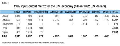
We calibrate most of the parameters of the U.S. portion of the model using an approach similar to that taken by researchers who use static, multisector applied general equilibrium models to analyze the impact of trade liberalization. (See, for example, Kehoe and Kehoe 1994.) We require that the model’s households, firms and government carry out the same transactions in the base year of 1992—the last year in which the U.S. current account was close to balanced—as do their counterparts in the data. Most of these transactions are summarized in the input-output matrix in Table 1, which we have constructed using data from the U.S. Bureau of Economic Analysis (BEA). In this matrix, each entry specifies the expenditures on intermediate inputs or factors of production (rows) made by the model’s three industries and final uses (columns). For example, the entry of 848 in the labor row of the goods column indicates that the goods sector paid U.S. $848 billion in labor compensation to households in 1992, and the entry of 3,346 in the services row of the consumption column indicates that households consumed U.S. $3,346 billion in services. U.S. gross domestic product (GDP) in 1992 was U.S. $6,342 billion, which is equal to the sum of consumption, government spending, investment and exports minus imports, which also equals the sum of labor income and capital income.
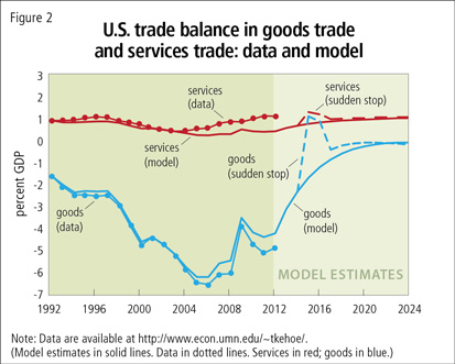
Our disaggregation of production into three industries—goods, services and construction—is not the typical one in international macroeconomics. Services and construction are usually aggregated into an industry called nontradable goods, while goods are called tradable goods. The table clearly shows that services are in fact traded, although they are not traded as much as goods. The table also shows that the United States had a large surplus in services trade in 1992, while it had a large deficit in goods trade. The time series data in Figure 2 show that this pattern persists over time. Our model closely matches this pattern between 1992 and 2012.
We use the empirical literature to set the model’s remaining parameters, the elasticities that govern substitutability: how substitutable goods consumption is for services consumption in the household’s utility function, for example, or how substitutable inputs of labor are for inputs of capital in production. Two other parameters—one for goods and one for services—govern substitutability between imports and domestic output for final uses. We choose these elasticities to be consistent with the higher volatility in the goods trade balance seen in Figure 2; that is, we assume that foreign goods are more substitutable for U.S. goods than foreign services are for U.S. services. Nonetheless, foreign goods are still imperfectly substitutable for U.S. goods in our model. That condition is how we are able to model the saving glut as driving down the relative price of foreign goods and forcing the U.S. real exchange rate to appreciate.
Our model of the rest of the world is simpler than our model of the United States. Firms in the rest of the world produce goods and services using linear technologies with labor as the only input; we abstract from capital formation, domestic input-output linkages and construction. Households in the rest of the world work, consume and save to maximize utility, and have similar preferences to their U.S. counterparts: They enjoy leisure and regard imports of U.S. goods and services as substitutes for domestic ones, with the same elasticity of substitution as in the United States. Households in the rest of the world can save or borrow only by buying or selling U.S. bonds.
The rest of the world’s intertemporal decision-making generates the saving glut. For 1992–2012, we calibrate the weights that the rest of the world puts on utility for consumption and leisure in different years so that it chooses to lend exactly enough to the United States to generate the trade balance dynamics observed in the data. During this period, the rest of the world discounts the future less than U.S. households, which induces it to postpone current consumption to be able to consume more later. It does so by buying U.S. bonds. After 2012, the rest of the world’s discount factor gradually converges to that of U.S. households so that the world economy converges to a balanced growth path in which the interest rate is 3 percent per year.
We model the sudden stop in 2015–16 in the same manner as Kehoe and Ruhl (2009), who model the Mexican sudden stop of 1995–96 as a surprise. Agents in the model have perfect foresight before the sudden stop occurs and afterward, but if and when the sudden stop occurs, it is completely unexpected. During the sudden stop, the rest of the world buys no more bonds, but households and the government in the United States make interest payments on existing bonds at the 2014 interest rate. The U.S. interest rate during the sudden stop is determined within the United States since there is no foreign lending.
We model the sudden stop as a surprise because U.S. interest rates currently indicate that financial markets do not assign a significantly positive probability to a U.S. debt crisis—just as they did not assign significantly positive probabilities to a crisis in Mexico in 1995 to or to the currently ongoing debt crises in the eurozone. (See, for example, Arellano, Conesa and Kehoe 2012.) We think of the possibility of a debt crisis striking the United States as the possibility of the sort of self-fulfilling crisis modeled by Cole and Kehoe (2000) and Conesa and Kehoe (2012).
The model incorporates additional data that are important in generating the equilibrium’s dynamics. We use projections from the UN World Population Prospects to model population growth in the United States and the rest of the world. To allow the equilibrium to converge to a balanced growth path, we assume that the population in the United States and the rest of the world converge to constant levels after 2050. We model U.S. government spending and borrowing to evolve over time using projections from the Congressional Budget Office (CBO). We use data from 1992–2011 on value added by sector to calculate annual productivity growth rates of 4.6 percent in goods, 1.4 percent in services and −1.3 percent in construction. We impose these growth rates over 1992–2030 and let productivity growth in each sector converge to 2 percent in all sectors thereafter.
Dynamics of the U.S. trade balance
Our model of the saving glut is designed to capture the impact of government policies in the rest of the world that may have been responsible for the saving glut, such as Chinese policies that discouraged consumption and promoted saving, or policies that kept the Chinese real exchange rate from appreciating against the U.S. dollar. It can also be seen as capturing factors that make saving in the United States more attractive for foreigners than saving in their own countries. (See, for example, Mendoza, Quadrini and Ríos-Rull 2007.)
Notice, however, that, besides modeling U.S. government spending and borrowing during 1992–2012, we do not model U.S. government policies such as monetary policies or policies to promote mortgage borrowing that may have been responsible for the massive U.S. borrowing during this period. See Obstfeld and Rogoff (2009) and Bernanke et al. (2011) for discussions of these policies and their interaction with the saving glut. We later argue, however, that it is unlikely that global imbalances over the period 1992–2012 were driven by lack of saving in the United States. That would imply that U.S. investment was low when, in the data, investment was high throughout this period.
Our view is that the saving glut is a temporary, albeit lengthy, phenomenon and that discounting of the future in the rest of the world will eventually revert to a value consistent with balanced growth. Bernanke (2005) takes a similar perspective:
“[T]he underlying sources of the U.S. current account deficit appear to be medium-term or even long-term in nature, suggesting that the situation will eventually begin to improve, although a return to approximate balance may take some time. Fundamentally, I see no reason why the whole process should not proceed smoothly. However, the risk of a disorderly adjustment in financial markets always exists.”
In other words, the current account imbalances associated with the saving glut will end eventually. The only question is whether the rebalancing process will be gradual or sudden.
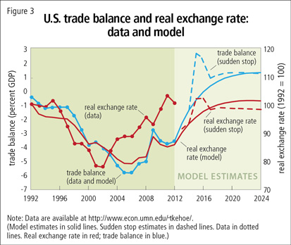
Figure 3 reports the results of two experiments, one with gradual rebalancing and the other with a sudden stop in new foreign loans to the United States in 2015–16. As explained, the model has been calibrated so that it exactly matches the U.S. trade balance in 1992–2012. The model matches the actual behavior of the U.S. real exchange rate during 1992–2002. In the model, the depreciation of the U.S. real exchange rate starts after 2006, while in the data it starts after 2002.
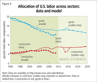
The model also captures much of the sectoral reallocation of labor during the saving glut, at least until the 2008–09 recession: In the data, workers in the goods industry received 19.7 percent of total U.S. labor compensation in 1992. By 2007, this number had fallen to 13.3 percent. In the model, the labor compensation that goes to workers in the goods industry goes from 19.7 percent in 1992 to 14.7 percent in 2007, capturing 78 percent of the decline observed in the data.
In construction, workers received 4.4 percent of total labor compensation in 1992 data, rising to 5.6 percent in 2007, the peak of the construction boom. In the model, reallocation toward construction is actually larger, going from 4.4 percent of total labor compensation in 1992 to 6.8 percent in 2007. The model does relatively poorly in capturing the collapse of the construction boom during 2008–12.
The intuition for the model’s performance is simple: During the saving glut, foreigners buy more U.S. bonds and less U.S. goods and services. To finance these bond purchases, the rest of the world sells its goods to the United States, lowering the relative price of these goods. The lower relative price of foreign goods shows up in appreciation of the U.S. real exchange rate. Since foreign goods are more substitutable for U.S. goods than they are for U.S. services and construction, as U.S. households and the U.S. government buy more foreign goods, they buy less U.S. goods and more U.S. services and construction.
In an experiment with the model in which the saving glut does not occur, labor compensation in goods falls from 19.7 percent of total compensation in 1992 to 16.2 percent in 2007, indicating that 70 percent of the drop in labor compensation in the model—and 55 percent of the drop in the data—is due to faster growth in productivity in manufacturing rather than to imports of foreign goods.
Notice in Figure 3 that, if a sudden stop occurs, it would have a very disruptive impact on the U.S. economy, causing the exchange rate to depreciate rapidly and the trade balance to move rapidly into a substantial surplus. Figure 2 shows that much of the improvement in the U.S. trade balance would come from goods trade because U.S. services are not very substitutable for services in the rest of the world. In Figure 4, we see that the U.S. construction industry would crash and its labor would be reallocated to goods and services production. In the baseline model that we are discussing, this reallocation is modeled as costless. In alternative specifications of the model with adjustment costs, the sudden stop is far more costly, echoing concerns expressed by Bernanke (2005):
“To repay foreign creditors, as it must someday, the United States will need large and healthy export industries. The relative shrinkage in those industries in the presence of current account deficits—a shrinkage that may well have to be reversed in the future—imposes real costs of adjustment on firms and workers in those industries.”
What do we learn from the model, and what do we still need to study?
As we can see in Figures 2, 3 and 4, our model captures four key features of the United States and its position in the world economy over 1992–2012: In the model, as in the data, the U.S. trade deficit first increases, then decreases; the U.S. real exchange rate first appreciates, then depreciates; the U.S. trade deficit is driven by a deficit in goods trade, with a steady U.S. surplus in service trade; and the fraction of U.S labor dedicated to producing goods falls throughout the period, with most of the drop due to higher productivity in goods than in services.
The performance of the model over 1992–2012 gives us some confidence in the predictions of the model for the future. The model predicts than the U.S. real exchange rate will depreciate as U.S households and government begin to repay the rest of the world. Much of the U.S. trade surplus will be in services trade and, if productivity in goods continues to grow faster than that in services, as it did over 1992–2012, employment in goods, particularly in manufacturing, is unlikely to ever return to its level in 1992.
These changes will occur whether the stop in foreign lending is sudden or gradual. A sudden stop in foreign lending, however, would be very disruptive to the U.S. economy. Construction, unlike goods and services, is completely nontradable, so it would absorb much of the shock of a sudden real exchange rate depreciation. During a sudden stop, the U.S. real interest rate would jump from 2.9 percent in 2014 to 5.5 percent in 2015. A sudden stop would cause a sharp contraction in output and employment in construction, more severe than the collapse of the U.S. housing boom in 2008–12.
A sudden stop would also change the welfare analysis of the global imbalances over the period 1992–2012. Twenty years of inexpensive foreign goods, as well as the credit with which to purchase these goods, has made U.S. households better off. We can calculate the increase in real income of U.S. households generated by the saving glut as being 1992 U.S. $689 billion, 10.9 percent of 1992 U.S. GDP.
If the saving glut were to end in a disorderly sudden stop, where productivity falls as it did in Mexico in 1994–95, however, these welfare gains would be lost and, in fact, U.S. households would suffer a real income loss of 1992 U.S. $330 billion, 5.2 percent of 1992 U.S. GDP, compared with a scenario in which the saving glut had never occurred. These calculations come from a model in which the costs of the sudden stop come from its surprise nature and from the drop in productivity; with adjustment frictions, the losses in real income would be larger.
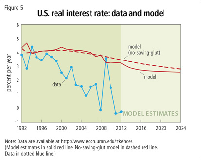
Our results leave a couple of puzzles that suggest directions for future research. In our model, the saving glut has only a small effect on U.S. interest rates, as seen in Figure 5, in contrast to Bernanke’s (2005) judgment. The largest fall the U.S. real interest rate in the model with the saving glut over 1992–2012 compared with the model with no saving glut is 46 basis points (3.70 percent per year compared with 3.24 percent) in 2009. This is in line with Greenspan’s (2005) judgment that foreign lending accounted for less than 50 basis points of the drop in interest rates. Warnock and Warnock (2009) have estimated that foreign lending drove down U.S. real interest rates by a somewhat larger amount, about 80 basis points, throughout the period.
In our model, the impact of the saving glut on interest rates depends on how substitutable foreign goods are for U.S. goods. With the elasticity of substitution parameter that we have chosen, we see that the saving glut generates the right magnitude of appreciation of the U.S. real exchange rate in Figure 3, but not the right magnitude in the drop in the U.S. real interest rate in Figure 5. If we make foreign goods more substitutable for U.S. goods, we can generate more of a drop in the U.S. real interest rate in the period 2006–12—although still nowhere near as large a drop as observed in the data—but the model would then predict a much smaller appreciation in the U.S. real exchange rate.
It is worth noting that our model predicts that the U.S. interest rate is driven up by appreciation of the dollar and is driven down by depreciation. The falling prices of foreign goods during the period 1993–2006 induce U.S. households to increase consumption faster than they do in the model without a saving glut, generating the observed trade deficit. U.S. households are willing to do this only if interest rates are higher. As the dollar depreciates during the period 2006–12, consumption grows more slowly than in the model with no saving glut and interest rates are lower.
Since our model does not provide a convincing explanation for the very low U.S. interest rates seen in the data, we need to look elsewhere, possibly at the sorts of U.S. policies discussed by Obstfeld and Rogoff (2009) and Bernanke et al. (2011).
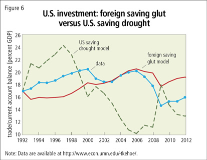
Modeling the source of the global imbalances over the period 1992–2012 as being generated by saving behavior in the United States, however, does not work well. We have followed Bernanke (2005) in modeling a saving glut driven by forces in the rest of the world. Alternatively, we could have modeled a saving drought in the United States in which U.S. households discount the future more than foreign households. Such a U.S. saving drought would generate the sort of increase in the trade deficit, real exchange rate appreciation and movement of labor out of U.S. goods production as the foreign saving-glut model.
This alternative model would generate very different results for U.S. investment during the period of global imbalances, however, as seen in Figure 6. In the data, the correlation between changes in the U.S. trade deficit and changes in U.S. investment is −0.79. In other words, U.S. investment increased as U.S. borrowing from the rest of the world increased. The foreign saving-glut model—where households in the rest of the world increase their saving—captures this relationship, and the correlation between changes in the trade deficit and changes in investment is −0.81.
The U.S. saving-drought model—where U.S. households decrease their savings—gets this relationship wrong, and the correlation between changes in the trade deficit and changes in investment is 0.82. The data indicate that the period of global imbalances was a period of increased investment worldwide—or consistent with the foreign saving-glut model, and not with the U.S. saving-drought model.
Although the model with a U.S. saving drought is successful in generating lower U.S. interest rates during the period 1992–2006, as the dollar appreciates, it generates higher U.S. interest rates during the period 2006–12, as the dollar depreciates. The low interest rates during the entire period thus pose a puzzle for both the foreign saving-glut and U.S. saving-drought models.
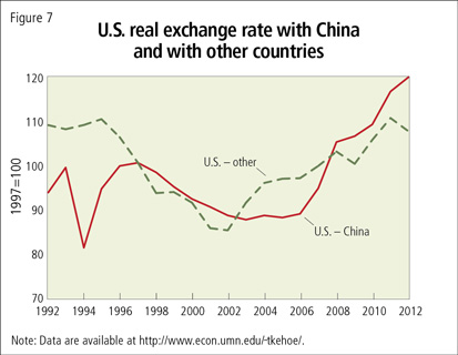
As we have mentioned, the timing of the depreciation of the U.S. real exchange rate is off in our model. It may be that the same factors that are missing from the model in capturing the low U.S. interest rates would also explain the U.S. continuing to borrow even as the real exchange rate depreciated. Disaggregating the U.S. real exchange rate suggests a simpler explanation, however: Figure 7 graphs the U.S.-China real exchange rate and the average U.S. real exchange rate against its other major trading partners. Notice that, starting in about 2001, as China became more important in trade with the United States, the real exchange rate in the model looks more like the U.S.-China real exchange rate. This suggests that we should explore models that consider countries like China, Korea and Japan—which are the principle lenders to the United States—separately from other U.S. trading partners.
We have performed extensive sensitivity analysis on the model. Our main results are robust to allowing agents to be uncertain about how long the saving glut would last. They are also robust to eliminating government borrowing and making government spending a constant portion of U.S. GDP.
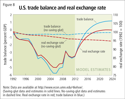
Our result that the long-term impact of the saving glut on the U.S. economy does not depend on how the saving glut ends does not say that the saving glut itself has not had a long-term impact. Figure 8 shows how large the long-term impact has been. The United States will have to run a substantial trade surplus in the future to repay its debt to foreign lenders. The purchasing power of the U.S. dollar—as measured by the reciprocal of the real exchange rate—will be lower. Output and employment in goods will be higher.
What should policymakers do?
Our results indicate that U.S. households have benefited from two decades of low prices of foreign goods, but that these welfare gains could be erased by a disorderly sudden stop in foreign lending. Policymakers should be vigilant to ensure that a sudden stop does not take the U.S. financial sector by surprise, as it was by the collapse of the U.S. housing market during the 2008–09 recession.
The need for prudential regulation in the U.S. financial system to prevent a sudden stop in foreign lending from becoming disorderly might seem to imply the need for capital controls. Recently, the debt crises in the eurozone have generated a renewal of interest in capital controls, especially in taxes on purchases and/or sales of assets by foreigners. See, for example, Farhi and Werning (2012) and Benigno et al. (2013).
The United States is in a unique position as the provider of the world’s reserve currency, however, and any attempt to impose capital controls on purchases or sales of U.S. assets—especially of U.S. government bonds—would push foreign governments to another currency, or currencies, for reserves. Indeed, much of the holdings of U.S. assets by the Chinese, Japanese and Koreans are in the form of U.S. government bonds. Since the United States enjoys substantial economic benefits from providing the world’s reserve currency, it is very unlikely, and probably undesirable, for U.S. policymakers to consider capital controls as one of the prudential regulations to guard against a disorderly sudden stop.
Note
* The authors thank David Backus, Kei-Mu Yi and Frank Warnock for helpful discussions. Participants at seminars and conferences made useful comments and suggestions. The authors are grateful to Jack Rossbach for extraordinary research assistance. The data presented in the figures are available here. The views expressed herein are those of the authors and not necessarily those of the Federal Reserve Bank of Minneapolis or the Federal Reserve System.
Endnote
1 We model households as paying taxes on capital income to be able to calibrate the model. Otherwise, we combine all the taxes and government transfers in the data into a simple tax that subtracts from household income in that year and does not depend on household decisions, a lump-sum tax. It would be useful to extend our analysis to capture the richness of the U.S. fiscal system, with distortionary taxes on labor, consumption, production and imports.
References
C. Arellano, J. C. Conesa and T. J. Kehoe (2012), “Chronic Sovereign Debt Crises in the Eurozone, 2010–2012,” Federal Reserve Bank of Minneapolis Economic Policy Paper 12-4.
G. Benigno, H. Chen, C. Otrok, A. Rebucci and E. R. Young (2013), “Capital Controls or Real Exchange Rate Policy? A Pecuniary Externality Perspective,” Inter-American Development Bank Working Paper IDB-WP-393.
B. S. Bernanke (2005), “The Global Saving Glut and the U.S. Current Account Deficit,” speech delivered at the Sandridge Lecture, Virginia Association of Economists, Richmond, VA, March 10.
B. S. Bernanke, C. Bertaut, L. P. DeMarco and S. Kamin (2011), “International Capital Flows and the Returns to Safe Assets in the United States, 2003-2007,” Board of Governors of the Federal Reserve System, International Finance Discussion Paper 1014.
H. L. Cole and T. J. Kehoe (2000), “Self-Fulfilling Debt Crises,” Review of Economic Studies, 67, 91–116.
J. C. Conesa and T. J. Kehoe (2012), “Gambling for Redemption and Self-Fulfilling Debt Crises,” Federal Reserve Bank of Minneapolis Staff Report 465.
E. Farhi and I. Werning (2012), “Dealing with the Trilemma: Optimal Capital Controls with Fixed Exchange Rates,” NBER Working Paper 18199.
A. Greenspan (2005), “Monetary Policy Report to the Congress,” statement before the Committee on Banking, Housing and Urban Affairs, U.S. Senate, February 16.
P. J. Kehoe and T. J. Kehoe (1994), “A Primer on Static Applied General Equilibrium Models,” Federal Reserve Bank of Minneapolis Quarterly Review, 18:2, 2–16.
T. J. Kehoe and K. J. Ruhl (2009), “Sudden Stops, Sectoral Reallocations and the Real Exchange Rate,” Journal of Development Economics, 89, 235–249.
T. J. Kehoe, K. J. Ruhl and Joseph B. Steinberg (2013), “Global Imbalances and Structural Change in the United States,” Federal Reserve Bank of Minneapolis Staff Report 489.
E. G. Mendoza, V. Quadrini and J.-V. Ríos-Rull (2007), “Financial Integration, Financial Deepness and Global Imbalances,” NBER Working Paper 12909.
M. Obstfeld and K. Rogoff (2009), “Global Imbalances and the Financial Crisis: Products of Common Causes,” CEPR Discussion Paper 7606.
F. E. Warnock and V. C. Warnock (2009), “International Capital Flows and U.S. Interest Rates,” Journal of International Money and Finance, 28: 903–919.


