Section 3: General Empirical Approach for the Capital and Leverage Tax Recommendations

This section discusses the general empirical approach we used to support our capital and leverage tax recommendations. For each of the recommendations, we summarize the relevant literature, describe our general methodology, identify key choices, provide key results and, where appropriate, discuss alternative approaches and/or sensitivity analyses. Section 4 walks through these calculations in detail.   As noted at the start of this Plan, the data and results in this paper are the same as those used in the November 2016 draft Plan unless otherwise noted.  Specifically, the November 2016 Plan was based on data on returns, loans, and risk-weighted assets through the end of 2015.  We did not update the results and figures because when we repeated the computational exercises with updated data, the results remained essentially unchanged.

3.1 Empirical Approach for the Minimum Capital Recommendations

This section reviews our approach for determining the higher minimum capital requirement we are recommending. We also review our approach for setting the SRC, which is an extension of the minimum capital charge approach. Our approach has one underlying tenet: Rely on existing analytical frameworks used by regulators or related groups to analyze the benefits and costs of higher capital requirements. At a very general level, this established approach calculates the benefits of higher capital as arising from fewer banking crises. The costs of higher capital come from increased costs of borrowing, lower investment and spending, and reduced GDP.

3.1.1 Relevant Literature.

In analyzing the benefits and costs of higher minimum capital requirements, we rely on the framework used by the Bank for International Settlements (BIS)—particularly BIS (2015) and work sponsored by the Financial Stability Board (FSB) (2015b), the Basel Committee on Banking Supervision (BCBS) (2010), and the Macroeconomic Assessment Group (MAG) (2010a,b)—and the International Monetary Fund (IMF). These analyses rely on a broad literature from both policy and academic sources.

To calculate the benefits of preventing a crisis, we follow the method used by IMF staff, specifically the work of Dagher, Dell’Ariccia, Laeven, Ratnovski, and Tong (DDLRT) published in March 2016. DDLRT approached the question of appropriate levels of bank capital by analyzing a data set of past crises from 1970 to 2011—the International Monetary Fund’s Systemic Banking Crisis Database (IMF database) compiled by Laeven and Valencia (2012). DDLRT compile average peak nonperforming loan (NPL) ratios for each crisis identified. By transforming the NPL ratios into equivalent capital ratios measured using risk-weighted assets, they infer levels of capital that might have prevented the need for the government intervention associated with these bank crises. The estimated capital levels are meant to indicate amounts sufficient to cover industry losses and maintain solvency for the representative banking systems.

The DDLRT analysis focuses on total capital held by a banking system in its determination of capital levels needed to avoid a crisis and bailout. We use these data to determine the capital level that covered banks should hold. This is a reasonable translation for two reasons. First, covered banks held approximately 70 percent of the total U.S. banking system assets as of year-end 2016. Second, some covered banks are so systemically important that their individual failure could cause a crisis. We want these banks to hold the level of capital needed to prevent such a crisis.

In contrast, we follow the BIS approach of assessing the cost of higher capital requirements quite closely. This analysis examined the cost of higher capital requirements through a two-step process. First, it estimated the impact of higher capital requirements on lending spreads. Second, it utilized central bank forecasting models to measure the impact of wider spreads on economic activity. We adhere to the same process and describe it more fully below. This framework is consistent with the literature that finds a negative relationship between capital and lending. (See Peek and Rosengren 1997, 2000.)

3.1.2 The Benefits of Higher Capital Analysis and Results.

In this section, we describe the general methodology we use, the key assumptions and choices we make, and our key results. We then report results from sensitivity analysis.

Methodology. The benefit of higher capital is the avoidance of a banking crisis and the related bailout of banks. The logic is straightforward. Banks with higher capital have a lower chance of failure, all else equal. The smaller the chance of bank failure, the less likely a banking crisis occurs. As noted, there is a one-to-one relation between banking failures and crises and public support for banks in the data we use. The lower the chance of failure and crisis, the lower the chance of bailout.

We implement this intuition by following DDLRT and reviewing the historical experience with banking crises. We use the IMF database to identify the number of crises that could have been avoided if the minimum capital requirement applied to banks in a country with a crisis was greater than or equal to the losses associated with those crises. The IMF database is set up for this exercise. It consists of banking crises that occurred between 1970 and 2011 and the NPL ratios for each of these crises. The data set has 105 crises with associated NPL rates.²³ Twenty-eight of the crises for which we have NPL data occurred in OECD countries.²⁴ The rest occurred in developing countries. Section 4 provides the technical details of implementing this general approach.

Key Choices and Assumptions. First, we rely on the historical record of banking crises. This raises two potential concerns:

1. Banking crises are tail events. Thus, we have few observations. This means we are considering what might occur in the future based on very limited history. As a result, our analysis faces a fundamental and unavoidable level of uncertainty. This challenge is endemic in all analytical efforts to prevent future crises, such as the supervisory stress test. We are trying to prevent events that simply do not occur very often; thus, we have limited experience with them. The BIS made this point in its analysis: “The benefits of prudential regulation are inherently uncertain and difficult to assess. Moreover, while in the case of regulatory capital requirements we can rely on historical evidence, we have only limited historical evidence that we can draw on to quantify the precise impact of TLAC and orderly resolution.” (See BIS 2015.)
2. We are assuming that the historical record regarding banking crises helps inform the future likelihood of crises. This assumption may not hold as well if the world has changed in some important ways relative to the past. Such changes could mean that the chance of having a crisis in the past no longer helps estimate the chance of having a crisis in the future. In particular, there have been a number of regulatory changes aimed at reducing the chance of a future crisis since the 2008 crisis. These changes may make it less likely that a banking crisis will occur in the future.

   Relying on historical data in this new world could thus overstate the chance of a future crisis. However, there are reasons to discount this concern with regard to our analysis. The historical data could understate future losses as well. Importantly, losses in the past reflect government bailouts to end crises. Losses in the past would have been higher if government had not stepped in. Some financial reforms since the financial crisis might also increase reported losses by, for example, forcing banks and supervisors to recognize losses earlier. Board of Governors analysis suggests that the overstatement of future losses and the understatement that arises from using historical crisis data may offset each other. The Board of Governors noted: “There are reasons to believe that the historical data underestimates the future trend and there are reasons to believe that those data overestimate the future trend. Although the extent of the over- and underestimation cannot be rigorously quantified, a reasonable assumption is that they roughly cancel each other out.” (See Board of Governors 2015a.) Moreover, this concern would apply to the reforms with which we are comparing our proposal, which also relied on the historical record. Finally, as already discussed, we are skeptical about the ability of some of the key reforms enacted to reduce the chance of a bailout.

Another key choice we make to help address the problem of limited data is to rely on cross-country data on financial crises to estimate the chance of a banking bailout in the United States. Of course, the U.S. economy and financial system differ from those of other countries. However, cross-country crisis data are the best information that analysts have for making such estimates, and we follow general practices in using them.

Next, we have to decide whether to use data on all crises, including those in developing countries, or a subset of that data. We use only the crisis data for OECD countries. We acknowledge that there are relatively few banking crises in the IMF database, and looking at a subset of crises makes our already sparse data even more limited. Nevertheless, we think it reasonable to conclude that future banking crises in the United States will be more like those that have occurred in OECD countries than in developing countries.

Another choice concerns the fact that higher capital requirements could make bank failure less likely in more than one way. Besides improving the ability of firms to absorb losses in the face of unexpected shocks, they could induce banks to take on less risk and thus face lower losses in the future. We decided not to account for this potential consequence of higher capital requirements. Instead, we account only for the loss-absorbing capacity of capital that makes failure less likely in the face of any given shock. We take this view because (a) the effect of higher capital on risk-taking of banks is not clear and (b) assuming that capital can only absorb losses rather than change behavior makes our estimates of benefits more conservative.²⁵

Finally, and on a more technical level, we decided to utilize the DDLRT cross-country NPL ratio information as a basis for understanding the size of loss for a given crisis. Like DDLRT, we ignore potential accounting differences and prudential requirements related to NPL ratios that could exist across countries.

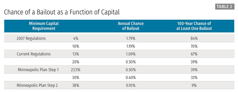
Key Results. Table 2 reports the key results of the benefits of higher capital using the methodology just described. In Table 2 and subsequent tables, we refer to probabilities of a bailout and costs of regulation associated with several minimum capital requirements over time. Before describing our results, we explain the source of the minimum capital requirement figures:

1. 2007 Regulations: We want to compare the effect of our proposal relative to prior capital regimes, including the precrisis capital regime. However, the pre- and post-crisis regimes have important differences in what they count as capital and the risk-weighting of assets. We use a 4 percent capital level to capture the precrisis regime. This is the precrisis Tier 1 capital requirement measured as a share of risk-weighted assets. On the one hand, this number overstates the amount of capital required relative to today’s regime because it counts as capital items that do not receive that treatment today. Moreover, the risk-weightings from the precrisis period are more favorable to banks than today’s. On the other hand, choosing the 4 percent level understates the minimum requirement because aspects of the precrisis system were akin to the capital buffers that we count in our current regulatory minimum figure noted below. We do not count those buffers—arising from the well-capitalized level of capital in the precrisis Prompt Corrective Action regime—in our determination of the precrisis minimum. In sum, this suggests that 4 percent is a reasonable selection, recognizing that there are inherent challenges in comparing pre- and post-crisis capital minimums.²⁶
2. Current Regulations: As of October 30, 2015, the TLAC proposal identified the maximum level of loss-absorbing capacity for the eight GSIBs to be 23.5 percent, which includes long-term debt of approximately 10.5 percent and common equity of 13 percent. Thus, we use 13 percent as the measure of current minimum capital regulation. This approach is conservative, as the requirement for most banks is below 13 percent.  Moreover, banks can take, and have taken, steps to reduce this minimum requirement. As described above, we consider only equity capital to be loss-absorbing, causing us to label the current regulation as a 13 percent target.
3. Minneapolis Plan Step 1: As described in Section 1, our proposal’s Step 1 target is 23.5 percent. We choose a level around this amount because of our benefit and cost analysis—a minimum capital level between 20 percent and 25 percent has substantial net benefits. (We describe how we determine net benefits in Section 3.1.4.) We choose the exact figure of 23.5 percent because it matches the reasonable amount of loss-absorbing financial resources that the Board of Governors determined the most systemically important covered bank in the United States should hold.
4. Minneapolis Plan Step 2: The level of capital that reduces the 100-year chance of a crisis below 10 percent using the IMF database is 38 percent.

Recall that the benefit of higher capital is the reduction in the chance of a bailout, which occurs when a banking crisis happens. We highlight three rows in Table 2. The first highlighted row reports the chance of a crisis and bailout in the next 100 years given the current minimum capital requirement of 13 percent (noted as Current Regulations). That chance is 67 percent. We then highlight the chance of a bailout in the next 100 years under our proposed minimum level of capital of 23.5 percent. The 100-year chance of a bailout under that regime is 39 percent. Finally, we highlight the chance of a bailout after Step 2 of the Minneapolis Plan, which is 9 percent.

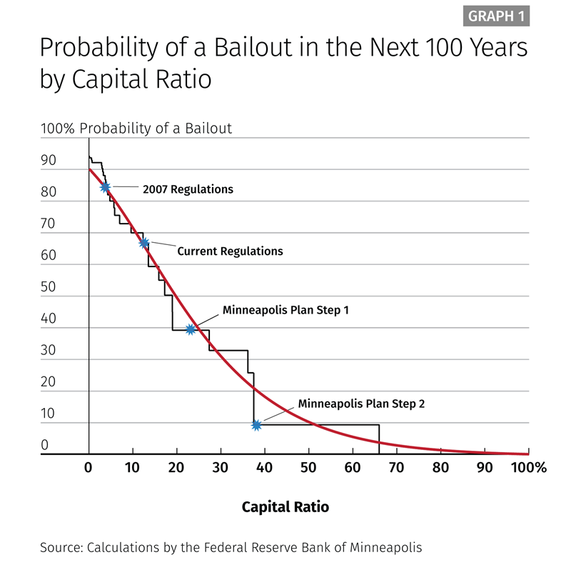
Graph 1 shows how a change in the capital ratio changes the chance of having a crisis and bailout. This graph also makes clear the limits of working with historical data on banking crises. The black line mapping the relationship between capital ratios is a step function, with portions of the relationship indicating that higher capital ratios would not reduce the chance of a crisis. This reflects the limited observations that are in the IMF data set.

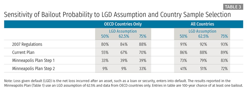
Alternatives/Sensitivity. The approach we take to calculating benefits comes with important inherent uncertainty for the reasons already noted. That said, it does not require many assumptions. Thus, there are relatively few variables for which we can choose alternatives to test the sensitivity of our analysis. We did choose to rely on crisis data from OECD countries rather than the full sample. Table 3 reports data if we use the full sample.

There is a relatively technical assumption in the calculation concerning the loss given default (LGD) of failing banks.²⁷ In this case, LGD is the amount of money that a bank loses when an asset, such as a loan or security, enters a state of default. LGD includes the amount that can be recovered. DDLRT cite research that examines recovery rates for securities and loans across different security types, industries, and macroeconomic periods. This work suggests that LGDs can range from 50 percent in normal periods to 75 percent in stressful periods. We take away from this literature that the choice of the LGD comes with much uncertainty, with many factors influencing the LGD. LGDs are higher for more-subordinated securities, for the financial industry, and during economic downturns. LGDs are significantly lower for loans than securities. Furthermore, accounting for industry differences generally removes the importance of economic cycles on the loss rates. Given a set of outcomes ranging from 50 percent to 75 percent across many sets of characteristics, we choose 62.5 percent as the LGD in our calculations, which is the average of 50 and 75. Table 3 provides details of the sensitivity of our probability calculations to this assumption.

Table 3 measures 100-year bailout probabilities for a set of minimum capital ratio targets for the two samples (OECD only and all countries) from the IMF data set. For each data set, the table reports values calculated under a low, medium, and high LGD assumption. Higher LGD choices tend to reduce the benefits of higher capital in these calculations.

The BIS used an alternative method to calculate the benefits of higher capital in the TLAC proposal. Some BIS calculations justifying higher capital levels find that, relative to our analysis, a lower level of capital would eliminate more future banking crises. Here we explain the differences between our approaches.

Our approach and the BIS approach for calculating the benefits of higher capital have important similarities. Both studies calculate the benefit as equal to the crises avoided by higher capital. Both studies also use the BIS figures for the dollar value saved by avoiding a crisis, which are based on the dollar value of lost GDP from a crisis. Moreover, we both use historical, cross-country data to determine the likelihood of a crisis based on how often crises occurred in the past.²⁸

However, we use a fundamentally different approach to calculate how higher capital reduces the chance of a crisis. The BIS looks to a range of models to convert the raw data into an estimate of how higher capital leads to a lower chance of a crisis. The BCBS also looks to reduced-form models, structural calibrated portfolio models, and stress test models to understand the influence of higher levels of capital. The BCBS considers a range of models and finds that 12 percent capital as a share of risk-weighted assets would be associated with a 50 percent chance of at least one bailout over a 100-year period.²⁹

We follow DDLRT and do not model this relationship. DDLRT simply calculate the losses associated with a given historical crisis. These losses determine how much capital would be necessary to avoid those crises. We choose the DDLRT approach for two reasons. First, we think the DDLRT approach is the most transparent and requires the fewest assumptions to determine the relationship between capital and the chance of a crisis. The BIS certainly provides details on its calculations. But we believe the DDLRT approach is much easier for an outsider to re-create and judge. Second, the direction of the worldwide regulatory community suggests that the lower levels of capital identified by earlier BIS analysis may be insufficient. In particular, the later BIS analysis behind the TLAC proposal uses a fundamentally different methodology to determine the appropriate level of loss-absorbing capacity for systemically important banks. That analysis supports a much higher level of loss-absorbing capacity than the earlier capital analysis would suggest.³⁰

We also note that some BIS analysis of the crisis data would support our recommended level of capital. In particular, a review of historical losses and recapitalization needs from the global financial crisis found that the maximum loss and recapitalization need for a systemically important bank was 25 percent of risk-weighted assets (in the case of Fortis). (See Financial Stability Board 2015b.) Our aim is to end TBTF. This goal suggests that we set our minimum capital level at the amount that would have prevented the failure of systemically important banks during the last financial crisis. Indeed, analysis of a broader set of historical banking/financial crises and related losses found that a loss-absorbing capacity of 24 percent of risk-weighted assets would be necessary to absorb the losses from 95 percent of banks.³¹ In a relatively similar vein, and even when limiting the analysis to the U.S. experience only, the Federal Reserve found that “the bank holding company with the most severe loss experience during the great financial crisis incurred estimated losses and recapitalization needs of roughly 19 percent of risk-weighted assets.” (See Federal Register 2015.)

The most recent, and in many cases the most rigorous, analyses of the benefits and costs of holding more capital have also supported our key capital recommendation. In particular:

• Passmore and von Hafften (2017) find that the most systemically important banks should face an extra capital surcharge of between roughly 7 percentage points and 14 percentage points on top of their current minimum levels of capital. This surcharge, at its upper ends, would bring capital to a level at or above the proposed minimum of the Minneapolis Plan.
• Firestone, Lorenc, and Ranish (2017, p. 1) conclude that “optimal bank capital levels in the United States range from just over 13 percent to over 26 percent,” with the higher range meeting or exceeding the Minneapolis Plan’s proposed minimum level.
• Egan, Hortacsu, and Matvos (2017, p. 170) report, “Our results suggest that capital requirements below 18 percent allow for equilibria with substantial probabilities of bank default and large welfare losses.” We find the analysis in Egan, Hortacsu, and Matvos (2017, pp. 204-06) to strongly support a capital requirement of right around 23 percent (as found in the Minneapolis Plan) and to potentially support a much higher level (e.g., around 39 percent) consistent with Step 2 of the Plan.
• Schnabl (2017, p. 44) reviews a wide range of analysis of minimum capital requirements and summarizes that “the required thresholds vary greatly across proposals with recommended capital ratios ranging from 9% to 30%. It is clear that all recommendations come with a number of assumptions on the economic magnitude of the costs and benefits of bank capital. Even though there is no unanimous consensus on the recommended level, none of the proposals recommends a number clearly below 10%, and most proposals recommend a number significantly above 10%. A prudent regulator may prefer a threshold that puts more weight on some of the higher estimates.”
• Barth and Miller (2017) find that increasing the minimum leverage ratio requirement to 15 percent—which matches our recommendation—passes a benefit and cost test.
• Perri and Stefanidis (2017, p. 3) find, “Quantitatively, however, to achieve a sizeable reduction in the probability of bailout, capital requirements should be increased significantly, in the 20% to 30% range.” They find that these results support the recommendation of the Minneapolis Plan but use a completely different methodology to obtain that result.

3.1.3 Describing the Costs of Higher Capital Analysis and Results.

To calculate the costs of our proposal, we follow the methodology of the BIS and the MAG as closely as we can. We describe the general steps we take under this approach in this section while providing the technical implementation in Section 4.

Methodology. The BIS/MAG approach has four main steps. First, the cost of any proposal reflects the amount of new equity capital banks must issue. So we start our analysis by comparing the amount of equity capital banks currently have relative to a target amount. For example, we compare current capital levels for covered banks with the proposed minimum level of 23.5 percent. The difference between the two is the amount of equity capital a bank must raise.

Second, we determine how much it costs a bank to fund itself with that much new equity capital. We use the following logic to determine the cost of the additional equity. The bank has the choice of funding itself with equity or debt. Debt is cheaper than equity in practice because banks can deduct the interest payments on debt, thus reducing their taxes, but they cannot deduct the dividends they pay on equity. Debt is cheaper than equity for other reasons, even if some models of how firms finance themselves suggest that the two have the same cost. We discuss this point shortly. We calculate the cost of equity as being equal to the return on equity that banks earn, while the cost of debt reflects the interest they pay on debt.

Third, we have to determine how banks respond to the higher costs associated with the larger share of equity funding and what that response means for bank customers and the overall economy. Following the BIS methodology, we assume that covered banks are able to pass through some of these higher costs in the form of higher rates on loans. Key questions are how much of the higher costs the covered banks can pass through and how banks that do not face the higher capital requirement respond. The BIS/MAG analysis assumes that banks pass through all of the additional funding costs to their borrowers. This could be justified if the market for loans were perfectly competitive and all banks were subject to additional capital requirements. But only the covered banks face a higher capital regime under our proposal. As a result, our base case is that banks can pass through only half of the higher costs. We discuss this decision below.

Finally, we must model how higher loan rates affect the economy. Higher loan rates should depress economic activity because they raise the cost of borrowing. Higher borrowing costs reduce investment, which should reduce GDP. But by how much relative to what would have occurred absent our higher capital requirement? To answer this question, we follow the BIS method and rely on models of the economy that central banks already use to simulate how a change in one part of the economy can affect another. In our case, we run such a simulation using the FRB/US model. FRB/US is produced and made available to the public by the Board of Governors.

Key Choices. Determining the cost of higher capital requirements using the BIS methodology is much more technical and requires many more choices than the calculation of benefits we described above. But we highlight two particularly important choices.

First, as mentioned, we must decide how much of the higher costs faced by banks get passed on to the economy as a whole. The BIS assumes that the entire amount of the higher capital requirement gets passed through to the economy. (See BCBS 2010, p. 2.) This result would hold in a perfectly competitive banking environment where all banks face the same capital requirements. This assumption seems extreme to us given that we are not imposing higher capital requirements on all banks. Moreover, while banks report that they face high levels of competition on a daily basis, they also report an inability to simply pass through all their costs (e.g., regulatory costs).

Alternatively, the Modigliani-Miller theorem would imply that the relative returns on debt and equity adjust and that bank funding costs are not affected by the higher capital requirement. Admati et al. (2013) strongly advocate for this approach. The tax benefits of debt as well as regulatory issues make it unlikely that Modigliani-Miller holds exactly (Cline 2015). We take a middle road and assume that banks can pass through half of the cost of higher capital as our main estimate. (We report how sensitive our results are to alternative pass-through rates below.)

Second, we must decide whether higher capital requirements for target banks lead to a temporary reduction in GDP or a permanent reduction. The BCBS primarily reports results under the assumption that higher capital requirements have permanent negative effects on output. (See BCBS 2010, p. 29.) However, it also considers the case of transitory effects, primarily through a “credit crunch.” If higher loan spreads persist indefinitely, as we assume, then the permanent-reduction approach seems the better option and is the one that we have taken.

Key Result.

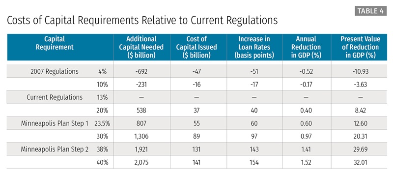
Table 4 reports the key inputs into our calculation of the cost of higher capital requirements as well as the ultimate estimated cost. Specifically, we report the amount of additional equity capital banks must issue, the cost of that equity capital, the amount by which estimated loan rates will change, and the impact on GDP associated with the adjusted loan rates. We report these cost data for a range of minimum capital requirements all relative to current regulations.  To summarize:

• Moving from the current regulations back to the 2007 regulations would reduce costs and increase GDP because the current regulations impose higher capital standards than the 2007 regulations.  The reduction in costs in this case is about 11 percent of GDP.
• Moving from the current regulations to the Minneapolis Plan Step 1 would increase costs and reduce GDP because Step 1 imposes higher capital standards. The increase in costs in this case is about 13 percent of GDP.
• Finally, moving from the Minneapolis Plan Step 1 to Minneapolis Plan Step 2 would increase costs and reduce GDP further because Step 2 imposes even higher capital standards. The increase in costs in this case is about 30 percent of GDP.

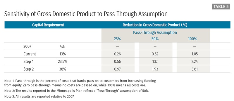
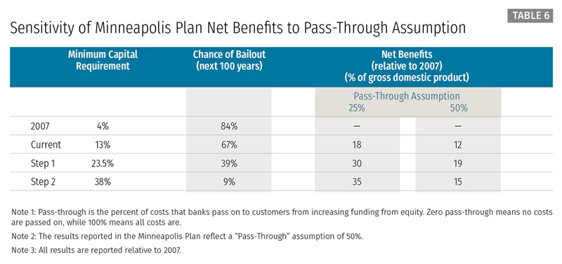
Alternatives/Sensitivity. We report how our results change if we alter the key pass-through decision discussed above. Table 5 reports how reductions to GDP would vary for our 23.5 percent minimum capital requirement if covered banks could pass through more or less than the 50 percent of higher loan rates that we assume. If they could pass through the full amount, the additional cost of our proposed higher minimum capital requirement would double from 1.12 percent of GDP to 2.24 percent. The cost of the proposal would fall from 1.12 percent of GDP to 0.56 percent if they could pass through only 25 percent of the higher funding costs. Table 6 replicates Table 1, comparing that table’s 50 percent pass-through assumption with results under the assumption that banks can only pass through 25 percent of their higher costs, which we consider to be more likely than the alternative of a 100 percent pass-through.

3.1.4 Comparing Costs and Benefits of Step 1.

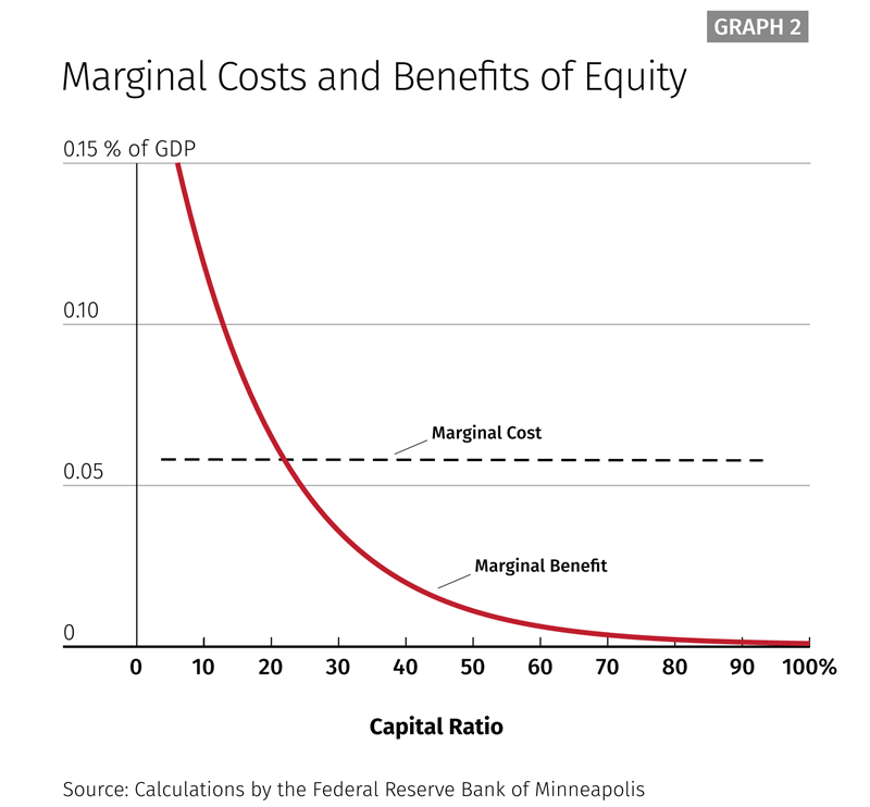
We noted when describing Table 2 that the 23.5 percent minimum equity capital requirement for covered banks has substantial net benefits. More technically, the 23.5 percent figure is near the point at which marginal benefits equal marginal costs. That is, the cost of one additional unit of capital is equal to the benefit of one additional unit of capital. The costs of higher capital vary (slightly less than) linearly with the required level of capital. As a result, the marginal cost of capital is constant and equal to 5.8 basis points of GDP per percentage point of capital and is shown as the straight line in Graph 2 below.

To calculate marginal benefits, we also have to express the benefits of additional capital in terms of output. This means we have to determine what constitutes a reasonable measure of the cost of a crisis. The cost of a crisis multiplied by the chance of a crisis gives us an economic value dollar figure for our benefit calculation. Here, too, we rely on the work of the BIS. As noted, we measure the cost of higher capital as its permanent reduction to GDP. We must measure the cost of a crisis in terms of its permanent reduction in GDP. The BIS finds this amount to be 158 percent of GDP in present value.³² The path of output after the most recent financial crisis looks very much like a permanent drop relative to the precrisis trend, and many observers consider that to be the case.

We noted above that our universe of historical banking crises is fairly small, and its distribution is a coarse step function rather than a smooth curve. We will not be able to compare marginal benefits to marginal costs effectively if we use a benefit “curve” that is a step function given that the cost curve is a smooth function. This means we must smooth the benefit data we use to make the marginal benefit and cost comparisons. We use regression analysis along the lines of Board of Governors (2015a) to perform this task.

Finally, we calculate the marginal benefits of higher capital as the incremental reduction in the expected loss of output from a financial crisis. The loss in the event of a crisis is assumed to be constant, but as capital increases, the probability of a crisis falls, but at a decreasing rate. As a result, the marginal benefit of additional capital decreases as the capital requirement increases. This is shown as the red line in Graph 2.

We then determine the point at which the marginal costs of higher capital equal the marginal benefits. Graph 2 shows the marginal benefit and marginal cost curves. The level of capital that sets marginal benefits equal to marginal costs is 22 percent. This is just a little below our Step 1 capital requirement of 23.5 percent, making our choice nearly optimal. Having reviewed our empirical approach for determining the 23.5 percent requirement, we then translate that figure into a 15 percent minimum leverage ratio. Our rationale and empirical method are described more fully in Appendix A.

3.2 Calculating the Systemic Risk Charge

3.2.1 Application of Step 2. Step 2 of our Plan provides covered banks with two choices, both of which should greatly reduce their potential need for a bailout. Covered banks can restructure or otherwise take steps such that they are no longer systemically important. The Treasury Secretary will determine if covered banks have reached that goal and will also have discretion to determine if other banks are no longer systemically important. If covered banks do not receive a designation as not systemically important, they will face a capital charge of up to 38 percent, which will be phased in over time. Each year a bank remains systemically important, an additional equity capital requirement of 5 percent of risk-weighted assets will be added to its Step 1 capital charge of 23.5 percent. The 38 percent charge is the point at which the 100-year probability of a crisis falls below 10 percent. At this point, the expected benefits still exceed the expected costs, but not by a large amount. Regardless, at our SRC of 38 percent capital, the likelihood of a financial crisis has been dramatically reduced from 67 percent to 9 percent. Put another way, going above 23.5 percent means that the additional costs exceed the additional benefits, but society is still better off than under current regulations.

We already noted that the 38 percent level for the SRC was chosen to reduce the chance of a bailout to 9 percent while passing a benefit and cost test.³³ In this section, we describe the process by which we think the Treasury Secretary will determine a firm’s systemic importance.

3.2.2 Determining Ongoing Systemic Risk of Designated Systemically Important Banks and Financial Firms.

Step 2 of our Plan gives firms a choice: Cease to be considered systemically important or face the SRC just described. Our Plan will charge the Treasury Secretary with determining if firms remain systemically important. Our charge for the Treasury Secretary regarding determining the systemic risk posed by banks and shadow banks differs from the current framework for assessing the systemic importance of financial firms. Today, the Dodd-Frank Act effectively determines which banks are systemically important, not the Treasury Secretary. The Financial Stability Oversight Committee (FSOC) determines which nonbank financial firms are systemically important.

In our proposal, the Treasury Secretary has responsibility for determining whether or not a bank or shadow bank is systemically important. The FSOC will not carry out its former role in designating nonbank financial firms as systemically important. Of course, systemic risk is inherently hard to measure. Thus, we provide the Treasury Secretary with the ultimate authority to make this determination. The Treasury Secretary can take advantage of the full range of data collection and analysis across the federal government to help identify and respond to systemic risk and financial instability.

The Treasury Secretary would not start the exercise with a blank slate. Bank supervisors, including the Board of Governors, use a set of metrics and measurements to assess the systemic risk posed by banks. They do so in the context of applying a so-called SIFI surcharge to GSIBs.³⁴ We would call on the Treasury Secretary to look to this measurement approach used by other regulators in determining whether or not a bank poses systemic risk. Of course, this need not be the only methodology, but it could contribute to the Secretary’s assessment.

Given that we recommend that the Treasury Secretary start with this approach to assessing systemic risk, it is worth noting that this approach generates a much smaller SRC than our proposal. Thus, we briefly describe why this outcome occurs. The Board of Governors’ analysis behind the calibration of the GSIB surcharge chooses an additional amount of capital to equalize the expected loss of a particular GSIB relative to a reference bank holding company that is not a GSIB in the event of a default.³⁵

Specifically, a higher capital level is sought for the GSIB to offset the fact that its default would impose more losses on society than a non-GSIB given its systemic nature. Mechanically, this approach attempts to reduce the GSIB’s probability of default by an amount that offsets its larger loss given default relative to a non-GSIB.

In the current period, the Board of Governors’ approach generates a capital surcharge roughly between 1 and 5 percentage points. As noted, our proposal would impose a much larger effective surcharge for banks deemed systemically important. A bank determined to be systemically important under our proposal could ultimately face a capital charge of up to 38 percent, which is about 15 percentage points higher than banks that the Treasury Secretary affirms are not systemically important.

This difference reflects the fact that we focus on trying to determine the level of equity capital funding banks need to reduce the 100-year chance of a banking crisis to 9 percent. As noted, we use cross-country data on banking crises to make this calculation. In contrast, the Board calibration relies on return on risk-weighted assets experience from large banks in the United States alone and over crisis and noncrisis periods. The use of nonstress periods in this exercise suggests that the tail outcomes may not be as extreme as those we are considering. We believe that continuing to focus on the distribution of outcomes from the IMF database is more appropriate and conservative. Specifically, the IMF database includes only financial crisis outcomes.

3.3 Empirical Approach for Shadow Banking Tax Recommendations

Setting a capital charge at the level we advocate raises concerns regarding nonbank financial institutions, or shadow banks, with which banks compete but which would not face the same capital standard. The big concern is that bank activities will move to the shadow banking sector, where they could receive less monitoring and fewer constraints. Over time, such movement could erode the ability of the new minimum capital requirement and SRC to end the TBTF problem. This activity could end up being funded with debt, and such leverage is a key source of risk that leads to spillovers. Thus, systemic risk will have shifted rather than declined.

We propose addressing this potential threat by levying a tax on borrowing in the shadow sector. This tax would try to make funding a balance sheet as costly in the shadow sector as in the banking sector. We would apply the tax to the borrowing of firms central to the shadow banking sector, with the determination of those firms informed by FSB analysis. Specifically, we would apply it to firms with assets greater than $50 billion. We would include off-balance-sheet assets and assets under management in that size definition given the centrality of off-balance-sheet activity to some critical shadow sector firms (e.g., asset managers). Of course, firms and investment vehicles with no borrowings would not pay the tax.

Taxing to discourage borrowing, or at least to not encourage it, in the financial sector is not an original idea (see the literature review below). But there is much less research on applying a leverage tax to the shadow banking system than there is on setting capital requirements. As such, we believe additional analysis and research on this aspect of our proposal will certainly improve it. This additional work would be particularly important for our proposal, as we take a very conservative approach that will impose the tax on borrowing even to firms that have high levels of equity capital.

3.3.1 Relevant Literature.

Our motivation for the shadow bank surcharge is related to, but different from, most analysis on banks, nonbanks, capital regulation, and taxes or surcharges. The main strand of the literature focuses on the tax-advantaged status of debt in most countries. The favorable treatment of debt in the United States, for example, encourages banks to take on more leverage (all else equal). Higher leverage raises the chance of bank failure. Moreover, bank failure can impose costs on society that bank owners and managers do not account for, leading to a classic externality problem. This outcome could potentially lead governments to eliminate the preferred status of debt for financial institutions and treat equity more favorably.

Roe and Tröge (2016a,b) argue that reversing the tax-advantaged status of bank debt would substantially decrease the risk in the banking system, allowing for less-stringent bank regulation. De Mooij and Keen (2016) find that favorable tax treatment of debt leads banks to take on more leverage as does Schepens (2015). Panteghini, Parisi, and Pighetti (2012) find that tax reforms in Italy to reduce the tax-advantaged status of bank-issued debt reduced leverage. Devereux, Johannesen, and Vella (2015) have a similar finding, but also report that higher asset risk-taking occurred at the same time leverage fell. Bengui and Bianchi (2014) and Begenau and Landvoigt (2016) examine formally the unintended consequences of regulation over the shadow banking system with the latter estimating an optimal capital charge across the banking and shadow sectors.

Our analysis has some overlap with the literature just summarized. We assume that banks will take on too much leverage under current capital regimes. By too much leverage, we mean that the chance of bank failure remains too high because of the external costs imposed by that failure. But we assume in the Minneapolis Plan that the government will force banks to internalize this externality through a higher capital charge. Thus, the problem is that activity previously conducted in the banking sector may move to the shadow banking sector, which does not face the same capital regime. In response, the government should set a charge that levels this uneven playing field.

In that sense, our review of the literature has focused narrowly on analysis of taxing borrowing in the banking system or at least not subsidizing borrowing in the tax code. There is a much broader and older literature on using taxes to discourage activity that poses spillovers, such as pollution. (See Barthold 1994 and Mankiw 2009.) 

There is also a separate and growing literature that examines the risk of the shadow banking system and seeks to limit and manage it using alternatives to a leverage tax. Some of the literature focuses precisely on the potential for higher bank capital requirements to move activity to the shadow sector. See Kashyap, Stein, and Hanson (2010) and Aiyar, Calomiris, and Wieladek (2014) for a discussion of this issue. Ricks (2016) argues for the use of entry restrictions to limit the potential for spillovers from the shadow banking system. Greenwood, Hanson, and Stein (2016) argue that government should issue additional money-like claims to crowd out the issuance of such short-term debt by shadow banks.

3.3.2. General Methodology.

Our approach, which we call the “funding equivalence method,” assumes that the new capital charge on banks is optimal and internalizes the externality caused by leverage per Bianchi (2011). The new, higher capital charge increases the overall cost of funds for the bank. The government should want the overall cost of funds in the shadow system to equal the new cost of funds in the banking system in order to level the playing field between sectors. We therefore calculate the charge on the shadow system cost of funds—in particular the costs of debt—so that the cost of funds in the shadow system equals that in the formal banking system. Thus, the shadow system also internalizes the externality of leverage.

We build on Bianchi (2011) by extending the analysis to allow for banks and shadow banks to fund themselves with equity, uninsured debt, and insured deposits. The basic intuition for this approach is as follows: The return on equity is greater than the return on debt, so financial firms would prefer to finance themselves with debt. In this approach, the level of debt without regulation (i.e., a tax on bank debt or a capital charge) is too high due to an externality.³⁶ The government can counteract the externality by imposing a tax on debt or, equivalently, imposing a minimum capital requirement for banks. Imposing a minimum capital requirement raises the costs of funds and reduces the amount of debt issued by the bank. This reduces the size of bank balance sheets to a more “socially optimal” level.

Under this framework, one can achieve the same “socially optimal” level by imposing a tax on borrowing of shadow banks. That is, given a minimum capital ratio, we can derive an equivalent tax rate for shadow debt borrowing. We take that approach in this section.

Section 4 contains the details of our calculations.

Finally, as a matter of administration, the revenues generated by the tax would not be earmarked for any specific purpose. That is, they would be considered general revenues. Moreover, we expect shadow banks subject to the tax to take steps to reduce or evade it. We would expect the agency that administers the tax to modify the rules implementing the tax and the methods by which they enforce it in response.  This approach should be the case with all well-administered taxes or levies today.

3.3.3 Key Decisions.

Implementing this approach requires many decisions.

First, we use this framework to calculate the tax rate that select shadow banks will pay on all their borrowings. But we could take an alternative approach. Some observers have noted that risk from shadow banks arises from their short-term borrowings. Holders of the short-term liabilities of shadow banks can run, equivalent to runs on banks by depositors. This would suggest that we tax only short-term borrowings of shadow banks. We decided to tax all borrowings for three reasons. First, consistent with an influential framework used by central banks to monitor risks to financial stability, we view leverage as a key source of systemic risk in addition to maturity transformation arising from borrowing short term and holding longer-term assets. (See Adrian, Covitz, and Liang 2014.) Second, we view long-term borrowing as posing its own risk. As noted, we think imposing losses on long-term debt holders of financial firms during periods of market stress can increase financial instability. Finally, by taxing all borrowings, we do not give up the imposition of an additional fee on short-term borrowings.

Second, we must also make a decision about the application of this approach—specifically, which firms will face the tax? To answer this question, we look to the existing literature on shadow banks to determine which types of firms should face the charge.³⁷  We follow the FSB’s policy framework for the oversight of shadow banks. (See Financial Stability Board 2013.) The FSB instructs authorities to “cast a wide net” and monitor all nonbank credit intermediation. The FSB also urges authorities to focus on activities and firms that increase systemic risk. Within their framework, the FSB begins by identifying nonbanks that engage in financial intermediation activities. It also monitors a narrower set of these firms that perform credit intermediation and have bank-like systemic risks. Thus, we choose to apply the tax to the representative firms that are identified and monitored by the FSB as a part of that narrower subset within its Global Shadow Bank Monitoring Report.

These entities are:

1. Funding corporations
2. Real estate investment trusts
3. Trust companies
4. Money market mutual funds
5. Finance companies
6. Structured finance vehicles
7. Broker/dealers
8. Investment funds
9. Hedge funds

Our approach does not put insurance firms into the group of shadow banks facing our proposed shadow banking tax. There are strengths and weaknesses with this decision. Supporting it is the view that insurance firms do not engage in the maturity transformation or reliance on short-term funding that typically generates systemic risk. That is, the business model of insurance firms does not justify them paying the shadow banking tax. However, the FSOC has deemed some insurance firms as systemically important institutions. And we know that insurance firms have the capability to engage in risky behavior, either in their core operations or in the form of activities ancillary to the provision of core insurance activities (e.g., AIG’s financial products activity).³⁸ The FSB’s summary material typically does not point to insurance firms as shadow banks. But we view additional analysis on the systemic risk posed by insurance firms as useful and important to determining if these firms should be subject to a shadow banking tax. Moreover, under our proposal, the Treasury Secretary would have the ability to determine whether to certify that a given nonbank financial firm, such as an insurance firm, is or is not systemically important.

Third, we must also decide if we want to target the tax to specific firms within these general groups. We think it makes sense to focus on the largest firms because they seem to have the most potential to pose systemic risk in the future. We choose a $50 billion asset threshold, which would include on-balance-sheet assets, off-balance-sheet assets, and assets under management. We choose this level because it is the cutoff in Dodd-Frank for determining which banks are systemically important. We fully recognize that choosing this threshold is arbitrary and may not ultimately prove to be the right level. Moreover, choosing a $50 billion threshold adds complexity to our proposal because this threshold is not the same as the one used for our capital regime for banks. We choose the lower threshold for shadow banks nonetheless because of the uncertainty in knowing which shadow banks pose systemic risk. The riskiness and threat to stability of shadow banks seem much less clear than they are for formal banks. As a result, we would prefer to err by including too many firms to face the shadow tax initially than too few firms. The agency setting the tax should work with elected officials to raise the asset threshold if it develops evidence that the threshold applies to firms it should not. In this same general sense, government agencies have adapted their application of rules over time to account for the fact that smaller firms facing those rules may not pose the same systemic risk as larger firms. It is also worth repeating that the tax applies only to firms that borrow. Firms of any size can escape the tax only by relying on equity funding.

Fourth, we assume that assets held by firms in both sectors are equally risky. This is a simplifying assumption to facilitate the calculation. It is difficult to determine the precise level of risk that assets in the two sectors pose. Thus, this seems like a reasonable assumption, but worthy of additional study and critique.

Fifth, we make this calculation assuming that shadow banks are not funded with any equity. In one sense, this is an extreme assumption. Many shadow banks are funded with very high levels of equity relative to commercial banks. Nonetheless, our Plan does not reduce its tax rate on borrowing in relation to any such equity levels. Why not? We want the tax to discourage shadow banks across the board from borrowing in the future to take on new activities that formal banks shed. As such, we set the tax high right away, avoiding the need to try to play catch-up once shadow banks have already leveraged up to formal bank levels. We also note an alternative approach below that would more directly take account of the equity of shadow banks in the setting of the tax.

3.3.4 Key Result.

Using our method, we estimate that the shadow banking surcharge should be 1.2 percent on the principal value of debt issued by shadow banks if a capital requirement of 23.5 percent was set on large U.S. banks in Step 1. As noted, shadow banks that continue to pose systemic risk would face a higher tax rate of 2.2 percent, which is equivalent to the SRC of 38 percent on covered banks.

We do not present an explicit comparison of benefits and costs of the shadow banking tax. That said, the benefit and cost analysis we conducted for banks is embedded in our shadow banking tax proposal. First, consider the cost of our proposal. The purpose of the shadow banking tax is to prevent intermediation activities from moving out of the regulated banking sector into the generally unregulated shadow banking sector after the higher equity requirement of Step 1 is imposed. As a result, the tax would raise the cost of funds for shadow banks, increasing the rates they would charge their borrowers, analogous to what would happen in the regulated sector. Our cost calculations do not distinguish the source of borrowing for nonfinancial corporations. So our calculations of the cost of equity already include the costs imposed by the shadow banking tax.

As for the benefits, we have insufficient data on the balance sheets of shadow banking firms. We have implicitly assumed that by limiting the growth of the shadow banking sector with the tax, we have prevented risk from moving from the regulated sector to the shadow sector. Thus, the benefits from the tax should be similar to the benefits from the higher equity requirement.

3.3.5 Alternatives/Sensitivity.

We considered three alternatives to our current approach.

First, an alternative framing of a tax on leverage in the shadow sector starts by noting the current practice of subsidizing leverage through the favorable tax treatment of debt. From this view, the first step is to eliminate this tax advantage before setting up a new tax. Our proposal effectively has that result. We would still generate a positive tax rate for shadow banks under our methodology, even if we assume the removal of formal banks’ and shadow banks’ tax preference for issuing debt. Put another way, our proposal has the effect of removing the tax preference for issuing debt in the course of also equalizing funding costs between banks and shadow banks. Specifically, eliminating the tax deductibility of debt accounts for 0.4 percentage point, or one-third, of the original 1.2 percent shadow banking tax. The remaining two-thirds of the tax serves to internalize the externality imposed by excessive borrowing.

Second, the tax rate could vary with the debt share of liabilities. Less debt would imply a lower tax rate. As equity increases from our assumed value of zero, the tax rate required to equalize the cost of funding across sectors falls. Given our choice of returns, a shadow firm with roughly 18 percent equity has the same cost of funds³⁹ with a tax rate of 0 percent as one of our covered banks or a shadow bank with no equity and a 1.2 percent tax on debt. Another alternative is a tax schedule that is an increasing function of a shadow bank’s leverage to induce firms to fund themselves with enough equity. The tax on debt would be very low, perhaps zero, for debt below 76.5 percent of liabilities. Above 76.5 percent, the tax on debt would be significantly above zero and perhaps even increasing in leverage. This would induce firms to satisfy the 23.5 percent equity requirement by their own choice. We chose not to pursue either of these approaches in the name of simplicity.

In a third and completely different approach, capital requirements could be set for shadow banking firms equal to the levels we propose for banks. In fact, we view this approach as attractive in concept as it is the most direct and does not require trying to relate a tax charge to a capital charge. But we do not view this potentially first-best option as available in practice. In particular, shadow banks exist across many industries, activities, and current regulatory regimes. It is not clear how practical it would be to set capital requirements equal given this institutional structure. Bank supervisors faced significant challenges in determining how to set capital levels for systemically important insurance firms. A tax would cut through this organizational and legal challenge. Our approach requires the government to try to equalize the cost of funding in both formal and shadow banking sectors. This is clearly difficult to do and comes with a high degree of uncertainty. Nonetheless, a tax seems more practical than the alternatives.

Endnotes

23 The IMF database consists of 147 banking crisis observations. Of those, 105 have associated NPL data. There are 29 OECD events reported in the database. All but one event has an NPL estimate.

24 See http://www.oecd.org/about/membersandpartners/ for a list of current OECD countries.

25 Calem and Rob (1999) find that higher capital requirements can lead banks to take on more risk.

26 As described in more detail in Section 4, we must use regulatory data on covered banks to complete the calculations. For example, we use data on capital levels and other bank holding company characteristics. We select those data as of year-end 2015. We use year-end data because they make our calculations more tractable with fewer assumptions and data manipulations.

27 DDLRT cite Schuermann (2004), Shibut and Singer (2014), and Johnston Ross and Shibut (2015).

28 There are a few differences in the data we use relative to the BIS/BCBS. The BCBS analysis includes data from Reinhart and Rogoff (2008). BCBS looks at data from 1985 to 2009, and they look at a different subset of countries than we do (countries in the “G-10 and countries that are members of the Basel Committee on Banking Supervision”).

29 See BCBS (2010, Table 3). We also note that the capital ratios target coming out of the BIS/BCBS analysis are based on a different definition of capital. This makes direct comparisons with our results more difficult.

30 The Financial Stability Board’s Impact Assessment assessed the benefits and costs of a TLAC requirement between 16 percent and 20 percent and found that the benefits exceed the costs. (See Financial Stability Board 2015b, p. 5.)

31 See the Vickers Report, available at http://researchbriefings.parliament.uk/ResearchBriefing/Summary/SN06171.

32 There is a potentially material but perhaps subtle implication of choosing this particular cost of a crisis figure in our calculation of benefits. We are implicitly assuming that avoiding a banking crisis means that other potentially related events that could also reduce GDP are also avoided. One could imagine that a shock to the banking system that leads to a crisis could independently also shock the rest of the economy. This scenario implies that the economy could have a recession even if the banking crisis is avoided through a proposal like our own. In that case, one would not want to count as a benefit the full reduction in GDP from avoiding a crisis because some fall in GDP might occur even if a crisis does not. We do not make an adjustment to account for this potential for several reasons; most importantly, our overriding strategy of trying to use existing analysis. The BCBS does not make this adjustment in its analysis. We also note that reductions in GDP due to a banking crisis may, in fact, be different from reductions in GDP associated with “regular” recessions. (See Reinhart and Rogoff 2008.) We look only to such banking-crisis related falls in GDP and not regular recessions.

33 Relative to current regulations, the benefits of this requirement continue to exceed the costs even assuming that all of the banks covered by Step 1 are also covered by Step 2. In this case, we mean total benefits and total costs, not marginal benefits and marginal costs.

34 For a detailed description of the charge, see Board of Governors (2015b).

35 The underlying data set comes from the Y-9C. It measures returns on risk-weighted assets for the largest 50 bank holding companies quarterly from 1987 to 2014.  (See Board of Governors 2015a.)

36 In the decentralized economy, the financial sector is “too big” in the sense that it issues too many loans to the nonfinancial sector (households) that are funded by borrowing on the world market. A tax on bank debt (or a costly capital requirement) raises the cost of bank loans, limiting the size of the financial sector.

37 We consulted work by the Federal Reserve, the Financial Stability Board (2014, 2015a), and the International Monetary Fund (2015). See also Adrian and Ashcraft (2012) and Pozsar et al. (2012).

38 Concerns about the systemic risk that insurance firms can pose can be found in Koijen and Yogo (2015, 2016).

39 The funding equivalence holds with 18 percent equity rather than 23.5 percent because shadow banks are not able to fund themselves with relatively low-cost insured deposits.